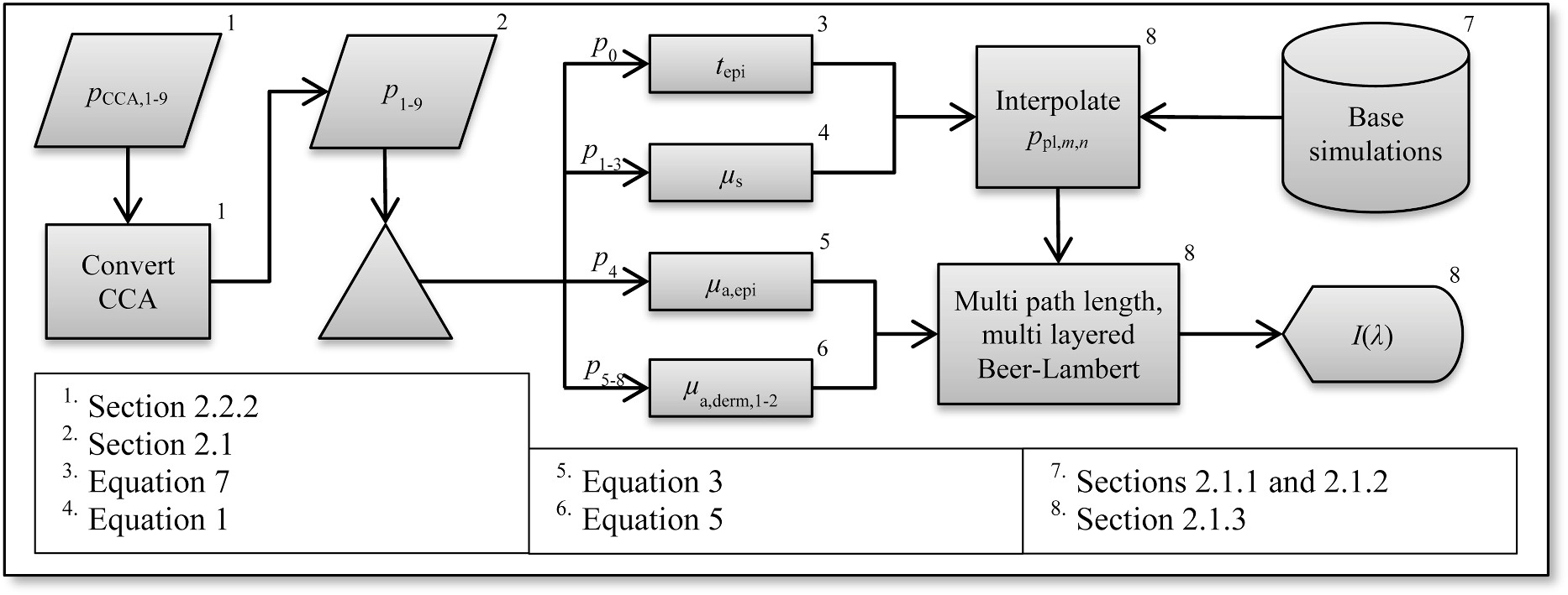
1.

Introduction

Diffuse reflectance spectroscopy (DRS) can be used for assessing tissue chromophores. Using white light in the visible to near infrared wavelength range and small source-detector separations will allow superficial sampling of tissue which is perfused mainly by the vessels in the microcirculation. Furthermore, in this wavelength range the absorption spectra of oxygenized and reduced hemoglobin show distinct features. This is advantageous for the determination of tissue oxygenation. With a model-based analysis of calibrated DRS, where knowledge on the absorption spectra of included tissue chromophores is assumed, quantitative measures of the chromophores can be attained.^1–4 For accurate estimations, this kind of model must include all chromophores of importance in the tissue, or else included chromophores will compensate for omitted ones.^1,5 Additionally, the fact that blood is confined to blood vessels and not homogeneously distributed must be taken into account.^6,7

For setups using small source-detector separations in the visible and near infrared wavelength range, where the absorption is on the same scale as the reduced scattering coefficient, diffusion theory fails to accurately describe light propagation. Instead, numerical simulations using Monte Carlo techniques provide a way to overcome these deficiencies. In addition, the Monte Carlo technique can be used to accurately model arbitrary complex structures.

It has previously been shown that a homogeneous model fails to describe the light propagation in skin at multiple source-detector separations in the visible wavelength range.⁵ This fact is a strong indication that a multilayered model should be used when analyzing DRS data from skin in order to accurately estimate the chromophore content. Both Wang et al.⁸ and Yudovsky et al.⁹ used Monte Carlo simulations of a two layered model in combination with a neural network analysis approach for estimating tissue optical properties (OP). Yudovsky et al. demonstrated that spatial frequency domain reflectance from a two-layered tissue model could be used for estimating dermis absorption and reduced scattering, while only epidermal optical thickness could be determined and this with limited accuracy. Wang et al. used spatially resolved diffuse reflectance and found that upper layer thickness improved upper layer OP estimation while lower layer OP accuracy deteriorated. These studies essentially determine OP using absolute calibrated reflectance at one wavelength but imply extension to spectroscopic use.

The approach proposed in this article differs in that it utilizes a subset of Monte Carlo simulated data for a limited number of tissue geometry and scattering parameters while adding the unique absorption characteristics of each chromophore directly in the inverse Monte Carlo algorithm. This is done by applying Beer-Lambert’s law on multiple path length-distributions in each layer in the forward calculation. Recordings were taken at two source-detector distances to make the method more sensitive to a layered structure of the tissue. The inverse algorithm is designed not to be sensitive to the average intensity detected at the two distances. This eliminates the need for an absolute calibration of the DRS system, which is difficult to perform accurately, and hence, eliminates the need for a well characterized calibration phantom that is stable over time.

The aim of this article is to present an inverse Monte Carlo method that uses a multilayered tissue model to estimate microcirculatory parameters in a diffuse reflectance spectroscopy setup. The accuracy of the method is evaluated using Monte Carlo simulations of tissue-like models containing discrete blood vessels. The performance of the method is compared to the performance of a similar method using a homogeneous model with absolute and relative intensity calibration. Examples of in vivo measurements are also given.

2.

Methods, Models, and Measurements

2.1.

Three Layered Bio-Optical Model

Photon propagation in tissue was modeled using Monte Carlo simulations of a three layered bio-optical model with nine free parameters. The design was based on previously presented models,^10,11 and consisted of one epidermal layer with a variable thickness $t_{\mathrm{epi}}$ (parameter 1) and two dermal layers where the upper had a fix thickness of 0.5 mm and the lower an infinite thickness. The scattering coefficient [${\mathrm{mm}}^{-1}$] was equal for all layers and was modeled as

Eq. (1)

$${\mu }_{\text{s}}=\alpha [(1-\gamma ){(\lambda /{\lambda }_0)}^{-\beta }+\gamma {(\lambda /{\lambda }_0)}^{-4}],$$

where $\alpha$, $\beta$ and $\gamma$ are given by parameters 2 through 4, $\lambda$ is the wavelength [nm] and ${\lambda }_0=600\mathrm{nm}$. The epidermis layer contained a fraction of melanin ($f_{\mathrm{mel}}$ [-], parameter 5). The absorption coefficient [${\mathrm{mm}}^{-1}$] of melanin was modeled¹² as

Eq. (2)

$${\mu }_{\text{a},\mathrm{mel}}(\lambda )=6.6\times {10}^{10}{\lambda }^{-10/3}$$

and the absorption coefficient [${\mathrm{mm}}^{-1}$] of the epidermis layer was modeled as

Eq. (3)

$${\mu }_{\text{a},0}(\lambda )=f_{\mathrm{mel}}{\mu }_{\text{a},\mathrm{mel}}(\lambda ).$$

The dermis layers contained different tissue fractions of blood ($f_{\text{blood},n}$ where $n$ is the layer number, parameters 6-7), where parameter 6 determines the average blood tissue fraction of the two layers and parameter 7 determines the relative ratio, $f_{\text{blood},\mathrm{rel}}$, between the layers. The same blood oxygen saturation was used in both layers ($s$ [-], parameter 8). The absorption spectra of fully oxygenated and deoxygenated blood¹³ (${\mu }_{\text{a},\mathrm{oxy}}$ and ${\mu }_{\text{a},\mathrm{deoxy}}$, respectively, hematocrit of 43%) are shown in Fig. 1 together with the absorption spectrum of melanin. The absorption coefficient of blood was given by

Eq. (4)

$${\mu }_{\text{a},\text{blood}}(\lambda )=s{\mu }_{\text{a},\mathrm{oxy}}(\lambda )+(1-s){\mu }_{\text{a},\mathrm{deoxy}}(\lambda )$$

and the absorption coefficients of the dermal layers were given by

Eq. (5)

$${\mu }_{\text{a},n}(\lambda )=f_{\text{blood},n}{c}_{\mathrm{vp}}(\lambda ){\mu }_{\text{a},\text{blood}}(\lambda ),$$

where $c_{\mathrm{vp}}$ is a compensation factor for the so called vessel packaging or pigment packaging effect caused by the inhomogeneous distribution of blood (located in discrete vessels rather than being homogeneously distributed in the layers). This factor depends on the average vessel diameter $D$ [mm] (parameter 9) according to Refs. 6, 7, and 14.

Eq. (6)

$$c_{\mathrm{vp}}(\lambda )=\frac{1-\exp [-D{\mu }_{\text{a},\text{blood}}(\lambda )]}{D_{{\mu }_{\text{a},\text{blood}}}(\lambda )}.$$

Fig. 1

Absorption coefficient of deoxygenized (blue circles) and oxygenized (red squares) blood with a hematocrit of 43%, and melanin (black diamonds).

Mathematically, the nine parameters $p_1\dots p_9$ were used to calculate the skin model parameters as:

Eq. (7)

$$t_{\mathrm{epi}}=p_1$$

Eq. (8)

$$\alpha =2^{p_2}$$

Eq. (9)

$$\beta =p_3$$

Eq. (10)

$$\gamma =p_4$$

Eq. (11)

$$f_{\mathrm{mel}}=p_5^2/t_{\mathrm{epi}}$$

Eq. (12)

$$f_{\text{blood},\mathrm{avg}}=p_6^2$$

Eq. (13)

$$f_{\text{blood},\mathrm{rel}}=2^{p_7}\times 8-1$$

Eq. (14)

$$f_{\text{blood},1}=f_{\text{blood},\mathrm{avg}}(1+f_{\text{blood},\mathrm{rel}})$$

Eq. (15)

$$f_{\text{blood},2}=f_{\text{blood},\mathrm{avg}}(1-f_{\text{blood},\mathrm{rel}})$$

Eq. (16)

$$s=p_8$$

Eq. (17)

$$D=p_9\mathrm{.}$$

Here, $t_{\mathrm{epi}}$ is the epidermal thickness in mm, $f_{\mathrm{mel}}$ is the volume fraction of melanin, $f_{\text{blood},\mathrm{avg}}$ is the average tissue volume fraction of blood, $f_{\text{blood},\mathrm{rel}}$ is the relative difference in blood tissue fraction from the average in the two dermal layers (ranging between $-1$ and 1), $f_{\text{blood},1}$ and $f_{\text{blood},2}$ are the volume tissue fraction of blood in the two dermis layers, respectively, $s$ is the fraction of oxygenated blood, and $D$ is the average vessel diameter in mm.

2.1.1.

Base simulations

Monte Carlo simulations were run for all combinations of six levels of the epidermis thickness ([mm])

Eq. (18)

$$t_{\mathrm{epi}}=x,x\in [0.0,0.1,\dots ,0.5],$$

and 12 levels of the scattering coefficients ([${\mathrm{mm}}^{-1}$])

Eq. (19)

$${\mu }_{\text{s}}=2^x,x\in [1,1.5,\dots ,6.5].$$

In total 72 simulations were thus performed.

A Henyey-Greenstein phase function with $g=0.8$ was used in all layers of the model. All layers had a refractive index of 1.4, whereas the refractive index of the source, detector and surrounding media was 1.5. The numerical aperture of the source and detector fibers was set to 0.37. All photons propagating outside a 5 mm radius of the source were terminated to increase simulation speed. In each simulation five million photons were detected between 0.01 and 1.8 mm from the pencil beam light source. The position of detection, photon weight and the path length in each layer was stored in the simulations.

2.1.2.

Path length distributions

When analyzing the base simulations, the pencil beam source was smeared out to mimic the size of the real fiber core by convoluting the detection positions with a circular area of 200 μm diameter.¹⁵ Two ring detectors were used, one between 0.3 and 0.5 mm (from the source), and one between 1.1 and 1.3 mm. The photons were re-weighted to reflect the detected intensity in a fiber rather than the ring detectors used in the simulations.¹⁶ Separate path length distributions were created for photons detected by these two detectors. For each detector, photons were grouped according to the deepest layer that they had reached. For each group, distributions were created over the path lengths that these photons had been propagated in each of the three layers. This resulted in a set of six distributions per simulation and detector: the distribution of path lengths in layer one for the photons that had only been propagating in layer one; the distribution in layer one for photons that had only been propagating in layer one and two; the distribution in layer two for the same photons; and so on. The resulting distributions (for one source detector separation) is denoted $p_{\mathrm{pl},m,n}$($d$) where $d$ is the path length, $m$ is the layer number and $n$ is the number of the deepest layer that the photon reached, $m\le n$. An example of the six path length distributions for the short source-detector separation (base simulation with $t_{\mathrm{epi}}=0.1\mathrm{mm}$ and ${\mu }_{\text{s}}=8{\mathrm{mm}}^{-1}$) is shown in Fig. 2.

Fig. 2

Example of path length distributions for detected photons that have only been propagating in the epidermal layer (a), only in the two uppermost layers (b) and in all three layers (c).

2.1.3.

Forward problem

The forward problem of calculating a model spectrum from the three layered model was based on interpolation of the path length distributions from the base simulations using Beer-Lambert’s law to add the absorption for each path length. We have previously described the important steps of this multi-path-length multilayered Beer-Lambert algorithm.¹¹

Initially, a set of path length distributions $p_{\mathrm{pl},m,n}$($d$) were interpolated linearly in two dimensions from the 72 base simulations, depending on the epidermis thickness of the model and the scattering coefficient of the wavelength of interest. From these distributions, the total intensity $I_{0,n}$ for photons that had reached layer $n$, was calculated as

Eq. (20)

$$I_{0,n}=\sum _d{p}_{\mathrm{pl},m,n}(d),$$

where $I_{0,n}$ is independent of $m\le n$. The path length distributions for varying $n$ were then normalized to unity

Eq. (21)

$$p_{\mathrm{pl},m,n}^{\prime }(d)=\frac{p_{\mathrm{pl}.m,n(d)}}{I_{0,n}}.$$

The path length distributions were modified for all path lengths $d$ by adding the absorption using Beer-Lamberts law

Eq. (22)

$$p_{\mathrm{pl},m,n}^{\prime \prime }(d)=p_{\mathrm{pl},m,n}^{\prime }(d)\exp (-d{\mu }_{\mathrm{a},m}),$$

where ${\mu }_{\text{a},m}$ is the absorption coefficient of layer $m$ [see Eqs. (3) and (5) for the epidermis layer and the dermis layers, respectively]. The detected intensity for all photons that had propagated down to layer $n$ and back was then calculated as

Eq. (23)

$$I_n=I_{0,n}\underset{m=0}{\overset{n}{\mathrm{\Pi }}}\sum _j{p}_{\mathrm{pl},m,n}^{\prime \prime }(d_j),$$

and the total detected intensity $I$ was then simply calculated as the sum of the $I_n:s$. The product in Eq. (23) follows from assuming that photon path lengths in one layer is independent of their path length in other layers. Even though this is an approximation, it only introduces insignificant errors in the modeled spectra.¹¹ With this assumption, a Monte Carlo-based technique that is sufficiently fast to be used in a real time inverse engineering approach with a multilayered model is introduced ($<1\mathrm{ms}$ for calculating a single 32-point spectra at the two source-detector separations with our implementation using an ordinary workstation).

The flow chart in Fig. 3 shows an overview of the forward problem.

Fig. 3

Flow chart describing the forward problem with references to relevant sections and equations.

2.4.

Validation Simulations

In order to test if a three layered model can be used to describe the light propagation in geometrically much more complex tissue, a set of 50 random validation models, all containing more than 100 individual blood vessels, were Monte Carlo simulated. By fitting spectra from the three-layered model to the spectra resulting from these simulations, the accuracy of the method could be evaluated. The details on how these models were randomly created can be found in the Appendix. These models consisted of an epidermis layer with a thickness varying between 0.045 and 0.47 mm with a melanin tissue fraction varying between 0.28% and 9.2%.

A semi-infinite nonabsorbing dermis layer was located below the epidermis layer. The dermis layer contained between 100 and 1750 infinitely long discrete blood vessels located with a random orientation parallel to the surface layer. The center positions of these blood vessels where randomly placed within a 3 mm radius of the light source. The blood vessels contained blood with a wavelength dependent absorption coefficient as given by Fig. 1, and the vessel diameters ranged between 6  and 160  μm. The blood vessel diameter generally increased with depth in the model. The oxygen saturation level of the blood in the vessels ranged between 0% and 100%.

The scattering coefficient was equal for both layers and modeled according to Eq. (1), with resulting values ranging between 1.1 and $17{\mathrm{mm}}^{-1}$. A Henyey-Greenstein phase function with $g=0.85$ in the epidermis layer and 0.7 in the dermal layer was used. The reduced scattering coefficient of the blood was set to $2.0{\mathrm{mm}}^{-1}$ for all wavelengths, and a Gegenbauer kernel phase function with $g_{\mathrm{Gk}}=0.948$ and ${\alpha }_{\mathrm{Gk}}=1.0$ (resulting in $g=0.991$) was used.¹⁰

The refractive index of both layers and the blood vessels was set to 1.4, whereas the refractive index of the source, detectors and surrounding media was set to 1.5. The numerical aperture of both source and detector was 0.37, the source had a diameter of $200\mathrm{\mu m}$ and the detectors were set to ring detectors 0.3 to 0.5 and 1.1 to 1.3 mm from the center of the source, respectively. For each of the 32 wavelengths, 150,000 photons were detected in total for the two detectors. A cross sectional view of one of the models is shown in Fig. 4.

Fig. 4

Cross sectional view of one of the validations models. The model contained 1275 vessels. The source can be seen as the middle rectangle, whereas the two ring shaped detectors constitute the other four rectangles at the top of the image.

In order to calculate the accuracy of the estimated RBC tissue fraction and oxygen saturation of the fitted three layered analysis model, we calculated the RBC tissue fraction and oxygen saturation within a $3{\mathrm{mm}}^3$ half sphere in the 50 simulated models. This calculation was done by randomly probing 15 million homogeneously distributed points within the $3{\mathrm{mm}}^3$ volume, and calculating the average RBC tissue fraction and oxygen saturation of these points. The $3{\mathrm{mm}}^3$ half sphere is marked in Fig. 4.

3.

Results

3.1.

Forward Calculation

We simulated a three layered model with RBC tissue fraction of 0.32% and blood oxygen saturation of 80%. The detected intensities at each wavelength were compared with the forward calculated spectra of the three layered analysis model with the exact same properties. The comparison is shown in Fig. 5. In this particular example, the relative RMS deviation between the simulated and forward calculated spectra was 1.0%.

Fig. 5

Examples of the spectral fit between the simulated (thick black) and forward calculated (thin red) spectra, 0.4 mm (a) and 1.2 mm (b) source detector separations. Corresponding residuals are also shown (c) and (d).

3.3.

Accuracy of RBC Tissue Fraction and Oxygen Saturation

3.3.1.

Three layered analysis model

The plots in Fig. 6 show the estimated RBC tissue fraction and blood oxygen saturation, respectively, compared to the values calculated from the $3{\mathrm{mm}}^3$ half sphere in the simulated models. The absolute RMS deviation between the true and estimated RBC tissue fraction was 0.087 percentage units and the absolute RMS deviation of the oxygen saturation was 4.2 percentage units (see also Table 1).

Fig. 6

Estimated RBC tissue fraction (a) and oxygen saturation (b) in fitted three layered models versus the same quantities calculated from the simulated models.

Half of the simulated models had an RBC tissue fraction $<0.3\%$. For these models, the absolute RMS deviation was 0.055 and 5.3 percentage units for the RBC tissue fraction and blood oxygen saturation, respectively. The relative RMS deviation for the RBC tissue fraction was 24% for these models. For the models with an RBC tissue fraction $>0.3\%$, the absolute RMS deviation was 0.11 and 2.9 percentage units for the RBC tissue fraction and blood oxygen saturation, respectively, and the relative RMS deviation for the RBC tissue fraction was 19%.

An example of the model fit is given in Fig. 7. The chosen spectra had the median ${\chi }^2$-deviation of all 50 models.

Fig. 7

Example of spectral fit (thin red) to spectra from simulated model (thick black) at 0.4 mm (a) and 1.2 mm (b) source-detector separations. Corresponding residual spectra are also shown (c) and (d).

3.3.2.

Homogeneous analysis model

The 50 simulated models were also analyzed using the homogeneous analysis model described in Sec. 2.3. The data was analyzed in three different ways: 1) a single detector using absolute calibration; 2) a single detector using relative calibration; and 3) two detectors using relative calibration. When the absolute intensity of a single spectrum was considered [1, merit function Eqs. (30) and (31)], the absolute RMS deviation of the RBC tissue fraction was 0.20 and 0.15 percentage units, respectively, analyzed for the source-detector separations of 0.4 and 1.2 mm. When the single spectra were relative calibrated [2, by using Eq. (30) in the merit function], corresponding numbers were 0.20 and 0.14 percentage units. These results should be compared to an RMS deviation of 0.087 percentage units for the three layered analysis model. Corresponding numbers for the RMS deviation of the blood oxygen saturation were 11 and 5.8 percentage units for absolute calibrated spectra and 12 and 5.3 percentage units for relative calibrated spectra, compared to 4.2 percentage units for the three-layer model. Paired t-tests indicated that the average deviation between estimated and true RBC tissue fraction and blood oxygen saturation was significantly ($p<0.01$) lower for the three layered analysis model than for the homogeneous analysis model at both source-detector separations. The estimated RBC tissue fraction and blood oxygen saturation from the homogeneous analysis model with absolute calibration are shown in Fig. 8.

Fig. 8

Estimated RBC tissue fraction (a) and oxygen saturation (b) in fitted homogeneous models versus the same quantities calculated from the simulated models.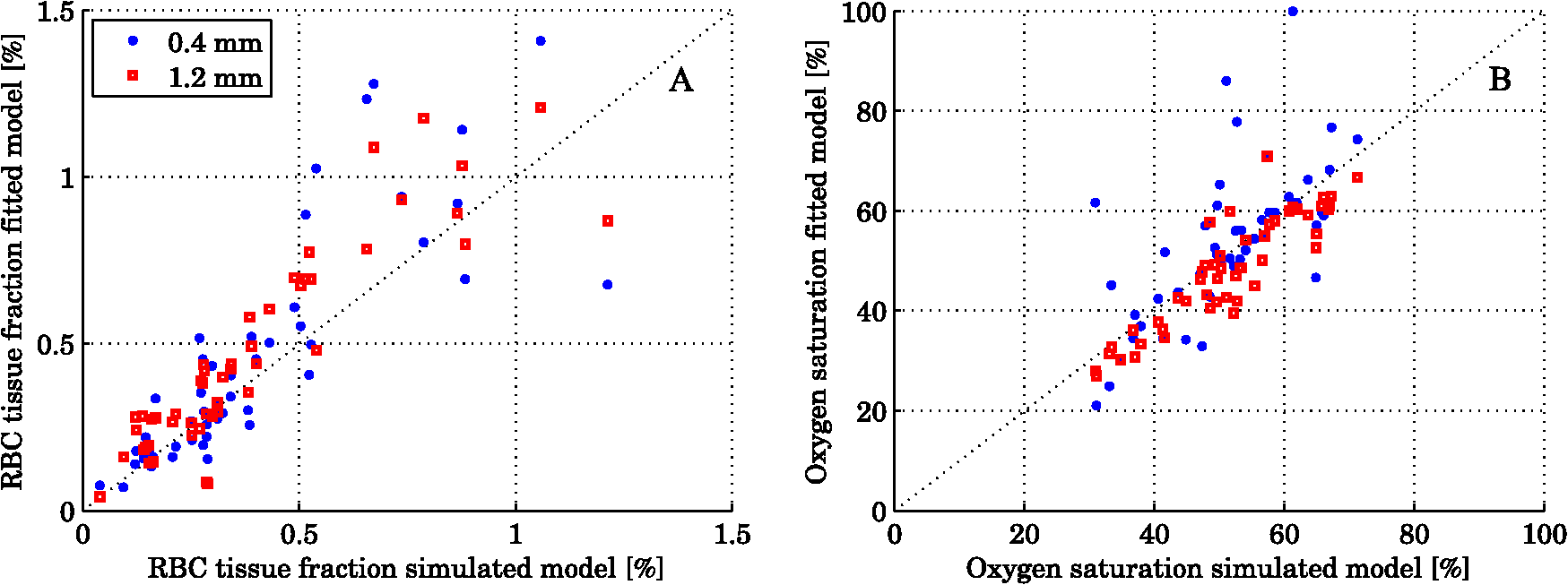

When using the homogeneous model and considering relative calibrated spectra at both separations (3), the spectral fit was poor (average spectral RMS deviation of 9.7%, compared to 1.3% for the three layered model), with obvious incorrect estimations of especially the blood oxygen saturation (RMS deviation of 30 percentage units).

3.4.

In Vivo Measurement

The RBC tissue fraction and blood oxygen saturation during the occlusion measurement are shown in Fig. 9. A slight increase in RBC tissue fraction can be noticed during the first minute of the occlusion, likely due to redistribution of blood to the venous side. As the pressure is released, a short peak is seen in the RBC tissue fraction, before it approaches the baseline. The blood oxygen saturation is slowly decreased during the occlusion, and a massive and quick increase is seen when the pressure is released, before it slowly approaches the baseline. Two examples of the spectral fit, at 0.5 and 3 min, are shown in Fig. 10.

Fig. 9

RBC tissue fraction (a) and oxygen saturation (b) during a provocation where the blood flow was occluded (between 1 and 4 min).

Fig. 10

Examples of the spectral fit between the measured (thick black) and fitted (thin red) spectra. Spectral fits are shown for the short (a) and (e) and long (b) and (f) source-detector separations at 0.5 (a) and (b) and 3 min (c) and (d). Corresponding residual spectra (relative deviation) are also shown (c, d, g, and h).

4.

Discussion

There are two key findings in this study. First, a three layered multi parameter tissue model is needed to explain spectra recorded at two separate source-detector distances in realistic simulated tissue models. The light propagation cannot be explained using a homogeneous tissue model. Secondly, when detecting the light at two distances from the source, a relative calibration routine, which only determines the relative intensity gain between the detectors, is sufficient.

The proposed method has an important advantage in the fact that it is not dependent on an absolute intensity calibration. An accurate absolute calibration is complicated to perform as it is sensitive to changes in the calibration standards, and thus error prone. Furthermore, when using an absolute calibration the inverse algorithm may become sensitive to measurement imperfections that are not included in the model but affect the two distances similarly, such as an air gap between the probe and the tissue and to intensity variations in the light source.³ The need for use of an index matching liquid is thus reduced, which facilitates the measurement procedure.

Simulated tissue-like models were used to determine the accuracy of the method, since controlled optical phantoms cannot be constructed with enough geometrically complexity. We have previously proven that it is possible to simulate homogeneous optical phantoms using a very similar measurement setup with high accuracy.²¹ Wang et al. managed to construct a two-layered semi-infinite tissue phantom⁸ with controlled OP, but still their tissue model was too simplified to mimic skin. The aim of the validation in this study was to test if a three layered model can describe the light propagation in a geometrically more complex, tissue-like, structure, and therefore optical phantoms were ruled out. In vivo measurements are improper for initial method validation since the exact expected values of the RBC tissue fraction and oxygen saturation cannot be determined, and the accuracy can thus not be evaluated. However, in vivo studies where the method is used are important to show the applicability of the method, and such studies are ongoing.

The three layered analysis model consisted of nine variable parameters. It was concluded that all nine parameters contributed to a significantly improved model fit in at least 28 of the 50 simulated tissue-like models. Based on the data presented in Table 1, it may be questioned if the parameters controlling the relative amount of blood in the two dermal layers and the average vessel diameter are necessary (significantly better fit in 28 and 39 of 50 spectra, but comparable RMS deviation in RBC tissue fraction and oxygen saturation). It should be noted, however, that in most of the 50 simulated models the blood tissue fraction does generally not differ much between superficial and deeper parts of the dermis, and the average vessel diameters are generally small compared to what can be expected in real tissue. In models where this was not the case, both the spectral fit and the estimation of the RBC tissue fraction were much worse when any of these parameters were excluded. The data in Table 1 also indicate the importance of not excluding any significant parameter; as doing so will cause the other parameters to compensate for the missing one. By omitting significant parameters the estimations of the RBC tissue fraction and oxygen saturation will be poor (see for example the column ${\chi }_{\gamma =0}^2$ in Table 1). The importance of not excluding any significant parameter has also been demonstrated in other studies.^1,5

In measurements on real tissue, the set of model parameters may need to be revised to better reflect the actual content and structure of the tissue under investigation and to improve the spectral fit. In epidermis and subcutaneous fat, beta-carotene has a nonnegligible absorption up to 500 nm.²² In blood, small amounts of bilirubin and met-hemoglobin are present and these concentrations may be high enough to have a significant influence on the diffuse reflected spectra in the visible wavelength range $<500\mathrm{nm}$ for bilirubin and between about 600 and 650 nm for met-hemoglobin) under some physiological conditions.^13,22,23 Water and fat are present in high amounts in tissue, but their absorption is negligible in the wavelength range used in this study (450 to 850 nm).^24,25 In muscle tissue, oxygenized and reduced myoglobin and cytochrome (c and aa3) both have significant effect on the diffusely reflected spectra. Myoglobin has absorption spectra rather similar to hemoglobin and it may be difficult to distinguish them. The cytochromes, which have characteristic absorption bands in the wavelength interval 500 to 650 nm, take a central part of the oxygen transport in the mitochondria in the cell, and monitoring their oxidation status is physiologically very interesting.^1,26 The same strategy as adopted in this study to determine model parameters that has a significant effect on the spectral fit can be adopted in clinical studies to determine which additional chromophores should be included when analyzing various types of tissue, and if any of the nine parameters included here should be removed. Studying Fig. 10, it may be seen that the spectral fit is relatively poor below 500 nm for the long fiber separation, a fact indicating that the model might benefit from the inclusion of bilirubin.

An alternative to the multi-path-length multilayered Beer-Lambert algorithm presented in this paper is to use a five dimensional look-up-table (LUT), where the five dimensions are constituted by epidermis thickness, scattering coefficient and absorption coefficient in the three layers, respectively. The LUT could be constructed from the same base simulations as used here, adding the effect of the absorption directly on each photon in a post processing step performed once (doing that for each forward calculation would be too slow). Using a LUT could even be faster than the proposed algorithm, but the absorption range in all three layers has to be restricted and the resolution in the absorption dimensions has to be fine enough over the whole range for accurate results.

One main focus during the development of the proposed multilayered inverse Monte Carlo technique has been to optimize the convergence properties. Equation (1) as well as Eqs. (7) through (17) are carefully chosen to ensure that the parameters affect the spectral shape in a somewhat linear manner over a wide range of parameter values, for example with the exponential in Eqs. (8) and (13), and the squares in Eqs. (11) and (12). Even if the parameters should affect the spectra in a perfectly linear manner, large correlations between how different parameters affect the spectra may exist. Such correlations have a negative influence on the convergence properties and should be avoided—such as by performing the canonical correlation analysis described in Sec. 2.2.2. Note that this type of de-correlation is not very efficient if the parameters affect the spectra in a highly nonlinear fashion.

When dealing with algorithms based on model fitting, one faces a possibility of rejecting models with a poor spectral fit to the measured spectra. One can also evaluate how sensitive the modeled spectra are to variations in the model parameters. If a parameter has a low impact on the model spectra, it is likely to be less accurately estimated. In both cases, one cannot assume that the fitted model reflects the actual quantities accurately. This is an advantage compared to methods that only calculate some type of index in the measured spectrum.

Other model parameters than the RBC tissue fraction and blood oxygen saturation may be clinically interesting in various clinical situations. Both the average vessel diameter and scattering parameters, obtained with related methods, has been used in studies involving various types of cancer.^27–30 The epidermal thickness, volume fraction of melanin and depth distribution of blood ($f_{\text{blood},\mathrm{rel}}$) may also be interesting, but before using any of these parameters as a clinical parameter, their accuracy should be evaluated. We have chosen not to evaluate the accuracy of these model parameters due to the fact that the method has been designed to estimate only the RBC tissue fraction and oxygen saturation accurately, especially when choosing the ${\chi }^2$-merit function (Sec. 2.2.1).

In conclusion, the three-layered analysis model is able to describe diffusely reflected spectra at two close but well separated source-detector separations simultaneously and is able to estimate the RBC tissue fraction and blood oxygen saturation more accurately than a homogeneous analysis model. An RMS deviation of 0.087 and 4.2 percentage units in the estimated RBC tissue fraction and blood oxygen saturation, respectively, was achieved on 50 simulated tissue-like models containing discrete blood vessels. No absolute calibration routine is needed for the method, and it is fast enough for real time analysis of recorded data.