|
|
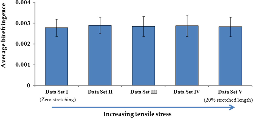
1.IntroductionAccording to the American Paralysis Association, the total annual cost of nerve repair exceeded $7 billion in the US in 2001.1 The National Center for Health Statistics found that more than 55,000 peripheral nerve injury repair procedures were performed in 1995.1 The primary causes of peripheral nerve injury are trauma, acute compression of the nerve, and various neurological diseases.2–4 The necessity for surgical intervention often depends on the severity of injury. In many cases, an injured nerve heals gradually in a short time and further surgical exploration is not required. Currently available methods to determine the condition of affected nerves include nerve conduction testing and imaging techniques such as MRI, ultrasound, and CT.5–9 Although current imaging methods have shown potential in providing images of the injured nerve as a whole, they lack the required submicron resolution to visualize damage or alteration to microstructures inside the nerve; moreover, they lack sufficient flexibility to quantitatively assess nerve health at different stages of the repair or treatment process.10,11 Optical coherence tomography (OCT) is a rapidly emerging imaging technology with applications in a range of fields including biology and medicine.12 OCT is capable of generating submicrometer-resolution cross-sectional images of biological tissues that can be readily assembled into 3-D volumetric reconstructions of the tissue sample. The ability to virtually slice down the sample to look at any desired cross-section without any physical incision is a significant reason for OCT to be thought of as an “optical biopsy.”13,14 In polarization-sensitive OCT (PS-OCT), the phase retardation between orthogonal polarization states of backscattered light is used as a source of image contrast, and it is useful for differentiating tissue types such as muscle, fat, and nerves.15–25 Nerve tissue is highly scattering in the near-infrared range of light, which results in a penetration depth of 1 to 2 mm below the tissue surface; however, this depth is sufficient in most occasions to get an image of the major portion of nerve and for quantitative characterization of desired structural features. A few earlier studies have demonstrated the use of OCT as an imaging modality for image-guided surgery26–28 and, more recently, for monitoring postinjury regeneration in the sciatic nerve following different types of trauma.29 Although these imaging studies provided valuable qualitative information on the nerve sample, there is a need for quantitative characterization of different structural features. In this article, we present quantitative imaging results of rat sciatic nerves using intensity-based regular OCT and polarization-sensitive OCT. Our goal was to quantitatively characterize the structural and relevant optical features of rat sciatic nerves to establish a control baseline for later studies with injured nerves. After a nerve injury, spontaneous nerve regeneration and repair largely depend on the preservation of internal microstructure.30 This becomes particularly important in the distinction between Sunderland’s 3rd- and 4th-grade injuries,3,31 where there is intact epineurium but internal structures are disrupted. Therefore, quantitative characterization of the axonal region inside epineurium and proper visualization of epineurium boundaries are critical for assessment of the injury site. The structural features and optical properties of rat sciatic nerve characterized in this study are (a) trace of nerve bifurcation, (b) epineurium thickness, (c) extinction coefficient and birefringence of both nerve and muscle tissue, (d) bands of Fontana,32–35 an optical effect seen due to the undulating nature of nerve fascicles, and finally (e) the effect on the birefringence of a nerve of stretching by longitudinal tensile stress. These results serve as a foundation for future studies on assessments of peripheral nerve injury as well as the nerve recovery process using OCT and its functional extensions. 2.Materials and Methods2.1.Sample Preparation: In Vivo and Ex VivoThe sciatic nerve of Sprague-Dawley rats (Charles River Laboratories, Wilmington, MA) was used as the animal model. Sprague-Dawley rats are widely used in peripheral nerve injury and recovery studies.36–38 This model allows for manipulation of a nerve of similar caliber and size to the human digital nerve and also forms a well-established basis for an objective assessment of motor function following injury. Eighteen rats were used for in vivo study, and one rat from this pool was used for ex vivo study. For birefringence and extinction coefficient measurement, data from all 18 rats were used. The Massachusetts General Hospital Institutional Subcommittee on Research Animal Care (SRAC) approved all procedures described. Anesthesia was an intraperitoneal injection of pentobarbital sodium (, Abbott Laboratories Chicago, IL). This was followed by surgical exposure of the right sciatic nerve via a dorsolateral muscle splitting incision. After in vivo imaging session was completed, the sciatic nerve from the rat for ex vivo study was excised and extracted for imaging. A series of volumetric data sets were acquired as a 2-cm length of nerve was stretched stepwise over approximately 4 mm. 2.2.Imaging: Data Acquisition and AnalysisA detailed description of our OCT system (Fig. 1) can be found in a previous report.25 Briefly, nerves were imaged using a spectral-domain OCT system with a center wavelength of 1320 nm and a FWHM of 68 nm. Light sent into the interferometer was first sent through an electro-optic polarization modulator to allow switching between orthogonal polarization states. A splitter split the light into sample and reference arms of the interferometer. Returning light from both arms passed back through the system and was sent to a polarization-sensitive spectrometer. The light was dispersed by a diffraction grating (1100 lines per mm) and split by a polarization beam splitter onto two 512-element InGaAs line scan cameras with a maximum line speed of 18.5 kHz. The axial resolution was 11 microns up to a depth of 1.0 mm, in good agreement with calculation based on the light source specification, and increased to 14 microns at a depth of 1.8 mm. The focused spot size of the scanning beam was 22.4 μm in diameter. The imaging depth was found to be 2.0 mm in air with a sensitivity dropoff of 8 dB over that range. A multithreaded software written in Microsoft Visual C++ running on a dual-processor computer managed data acquisition and updated displays for spectrum, intensity, polarization, and flow, as well as saved data to the hard disk for postprocessing of images. Fig. 1Diagram of the multifunctional 1310-nm SD-OCT system. pbs, polarizing beam splitter; pm, polarization modulator; oc, optical circulator; , fiber splitter; pc, static polarization controller; ndf, neutral density filter; , transmission grating; pol, polarizer; lsc, line scan camera; DAC, data acquisition computer. 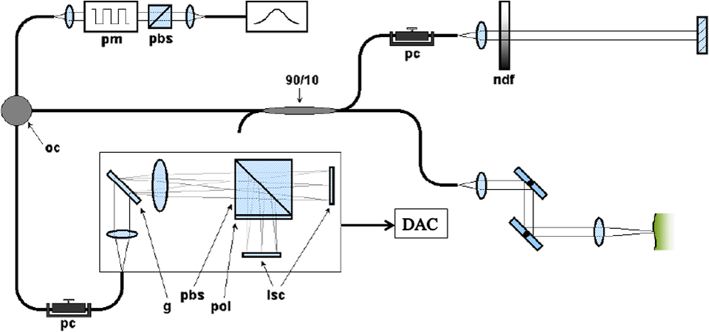 Raster scanning of the sample arm was performed with the fast axis perpendicular to the long axis of all nerves, with each scan resulting in a cross-sectional image of the nerve. Each intensity cross-sectional image comprised 2048 depth profiles that spanned a physical width of 5 mm. Polarization cross-sectional image of the same cross-section was simultaneously generated. Within the 5-mm length of the nerve sample, 200 frames were acquired, and these frames altogether constituted a 5- by 2- by 5-mm volume. Scanning and acquisition of this nerve volume required 22 s for 200 frames of 2048 depth profiles at a rate of 18,500 Hz. Each image was processed individually using Matlab® 2009b in a graphics-processing unit (GPU)-enabled multicore processor computer. Image processing techniques similar to an earlier study19 were followed for both intensity and polarization information. Volumetric reconstructions from these cross-sectional images, both intensity and polarization, were compiled using a visualization software package (Amira, Visage Imaging Inc.). 3.Results3.1.Structural Imaging and Volume RenderingIntensity-based OCT image of an ex vivo nerve cross-section and volumetric reconstruction from such intensity images are shown in Fig. 2(a) and 2(b). In intensity images, black and white color represent high and low back-reflected light intensity, respectively. Figure 2(c) and 2(d) shows corresponding polarization-sensitive OCT images of the same sample. A Stokes vector approach was used in calculating phase retardation for these images; the details of this method are explained in our previous studies.19,25 In phase-retardation images, black color represents zero phase retardation and white color represents 180-deg phase retardation. Fig. 22-D cross-sectional images and 3-D reconstructions of a 5-mm section of the rat sciatic nerve ex vivo. (a) A representative 2-D cross-sectional intensity image. (b) 3-D volume reconstruction of nerve from 200 intensity images taken along the 5-mm length. (c) A representative 2-D cross-sectional phase-retardation image. (d) 3-D volume reconstruction of nerve from 200 phase-retardation images taken along the 5-mm length. Scale bar, 200 μm. 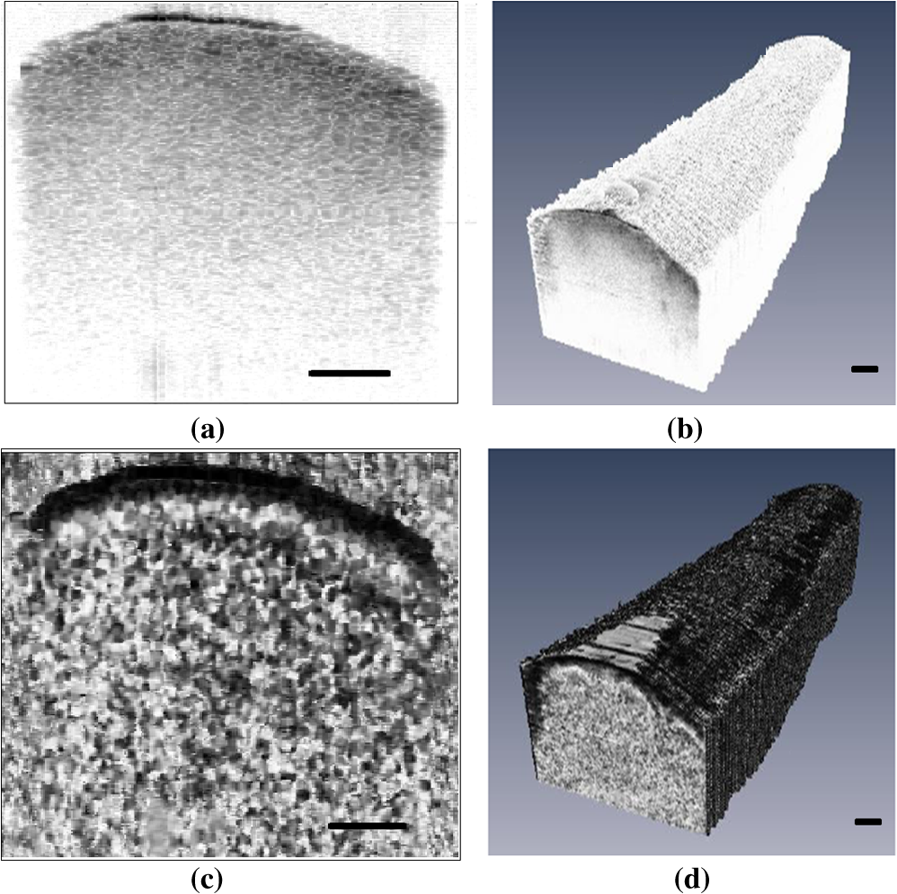 Quantitative analysis of these OCT images was performed to extract structural features using different image-processing techniques. The results of analysis are organized in the following manner: (1) visualization of a nerve bifurcation in generated OCT images, (2) visualizing epineurium with its inner and outer boundaries, measuring the epineurium thickness and the variability in thickness as a function of nerve stretch, (3) in vivo characterization of nerve and muscle optical properties—extinction coefficient and birefringence—as a means to distinguish these tissues from each other, (4) 3-D visualization of bands of Fontana and measurement of frequency of bands to quantify the effect of nerve stretching, and (5) measurement of average birefringence in a nerve ex vivo as a function of stretch to demonstrate that stretching a nerve does not lead to a significant change of birefringence. 3.2.Visualization of Trace of Nerve BifurcationA slight bifurcation was observed in the ex vivo nerve sample. During the OCT imaging session, the trace of this bifurcation could be seen in both intensity and phase-retardation images. Figure 3 shows the intensity and phase-retardation images of a cross-section at the bifurcating end of the nerve. A notch (gradually increasing along the long axis of the nerve) starts to appear at the location of bifurcation in both images, indicating that the nerve is bifurcating into two smaller nerves, which are starting to form their own epineurium (notch shown by arrow). This ability to visualize nerve bifurcations can be used to properly localize OCT images along a length of a nerve. Fig. 3Trace of bifurcation visible in both 3-D intensity volume image (a) and 3-D phase retardation volume image (b) of an ex vivo sciatic nerve sample (arrow). In (c) and (d), intensity and phase-retardation cross-sectional images are shown that represent the area of dotted lined planes in (a) and (b), which are perpendicular to the long axis of nerve. Arrows in (c) and (d) indicate the mark of bifurcation notch, and the horizontal line indicates the depth at which the volume images are displayed in (a) and (b). Scale bar, 200 μm.  3.3.Quantitative Measurement of the Epineurium of Sciatic NerveThe epineurium is a layer of connective tissues that surrounds peripheral nerves. One of the objectives of this study was to measure the thickness of this outer layer and define its boundary so that the relative position of axons and mesoneurium with respect to epineurium can be easily visualized. The middle 50% of the nerve was used for quantitative analysis in both intensity and phase-retardation images to minimize artifact from associated connective tissues on both sides of the nerve. The curvature of analyzed nerve surfaces was flattened such that pixels in each depth profile represented the same physical depth below the surface of the nerve. These adjusted depth profiles were averaged to get an average depth-resolved intensity profile for each sample. Given the anatomy of a peripheral nerve, with an outer epineurium surrounding bundled axons, it can be expected that the axonal region has uniform decay with depth, especially when depth profiles over a lateral width larger than perineural bundles are averaged together. Intensity OCT data is typically displayed on a logarithmic scale, so the expected exponential decay of backscattered light intensity within this region will appear as a linear decrease in the averaged depth profiles shown. We fitted the uniformly scattering region of the curve in Fig. 4(b) with a linear fit and extrapolated that linear fit for the entire plot. The absolute value of residuals (or offsets) between the linear fit and actual curve are calculated and plotted separately in Fig. 4(c): a threshold line is drawn (dotted line) based on the residuals obtained only from the linear-fit region of the curve ( standard deviation of residuals from linear portion). From the plot in Fig. 4(c), the amount of residual initially exceeds the threshold and begins to be smaller than the threshold after a certain tissue depth. We considered the first intersection of residuals curve and threshold line as the outer line at which the uniformly scattering interior of the nerve meets the outer sheath. This outer line is used as the marker of epineurium posterior boundary, and the top surface of nerve (marked by an arrow) is considered as the anterior boundary. Following this assumption, the thickness was calculated for all intensity data sets for that ex vivo sample. Fig. 4OCT images and data analysis for measurement of epineurium thickness. (a) Cropped middle 50% of the nerve from a 2-D cross-sectional intensity image. (b) Average intensity depth profile from the selected region of nerve; the arrow indicates the top surface of nerve. A linear fit is drawn based on the linear portion of the intensity curve and extrapolated on both sides. (c) Residuals or differences between linear fit and actual intensity curve are plotted and compared with the threshold line. The first intersection is considered as the posterior boundary of epineurium. (d) Cropped middle 50% of the same nerve from a 2-D cross-sectional phase-retardation image. (e) Average phase-retardation depth profile from the selected region of nerve. The slope of the rising portion is usually used to calculate the birefringence of the nerve area inside the epineurium. The blue curve is the phase-retardation plot calculated in Stokes-based method. Inset shows a comparison between phase-retardation plots calculated from both Stokes-based method (blue) and Jones matrix analysis (red). The slopes are of similar order. (f) Residuals or differences between linear fit and actual phase-retardation curve are plotted and compared with the threshold line. The intersection is considered as the posterior boundary of epineurium. Scale bar in (a) and (d), 200 μm.  To measure the epineurium thickness from phase-retardation images, a slightly different technique was used. An average depth-resolved phase-retardation profile from the middle 50% of a nerve in a phase-retardation image [Fig. 4(d)] is plotted in Fig. 4(e). With a similar assumption that the interior portions of the nerve will have uniform optical properties different from those of the outer sheath when averaged over this width, we can determine the epineurium thickness through differences in birefringence, or the slope of the depth-resolved phase retardation. We can therefore do a linear fit of the phase retardation within the axonal region [Fig. 4(e)]. Near a depth of 0.22 mm, a phase-wrapping artifact25 can be observed. Up to this point of our analysis, all phase-retardation calculation was done using Stokes method; the range of measurable phase was . To verify the homogeneity of the overall axonal region, we also used Jones matrix analysis, which can measure phase in range , of the same data. After unwrapping the phase, we found that a similar slope was maintained up to a depth of 0.3 mm [inset in Fig. 4(e)], and beyond that depth, the intensity became too low to reliably measure the phase retardation. (We found that minimum SNR required for reliable phase information is 25 dB in this study; hence, both intensity and phase-retardation curves are shown in broken lines where SNR becomes less than 25dB.) A linear fit was used to get the slope of the rising portion in the phase-retardation curve, and the slope was extrapolated for the entire plot. The residuals between the linear-fit and actual phase-retardation curve are plotted in Fig. 4(f). The posterior boundary of epineurium was determined as the depth at which the difference between linear fit and actual phase curve began to be smaller than the threshold value (mean standard deviations of residuals from linear portion). As before, the top surface of nerve was considered as the anterior boundary. Following this assumption, the thickness was calculated for all data sets. Epineurium thickness values obtained using these two methods are summarized in a column graph in Fig. 5. Average epineurium thickness from intensity images was found to be (mean standard deviation). In comparison, the average epineurium thickness from phase-retardation images was found to be . The analysis was repeated for stretched (nerve under longitudinal tensile stress, stretched gradually up to 20% of its original length) and unstretched nerves, and no significant difference in epineurium thickness was observed (Fig. 5). The measured values agree well with previously reported measures of rat sciatic-nerve epineurium thickness.39,40 3.4.Differentiating Nerve Tissue from Muscle Tissue In VivoFor in vivo applications, even before detailed investigation of the nerve, it is important to differentiate nerve from other associated tissues, such as muscle, fat, etc. In this in vivo part of the study, the sciatic nerve and associated tissues of 18 rats were imaged using OCT. The scanned regions contain nerve, muscle, fat, and some connective tissues as well. These images were later processed to characterize different tissue types by determining their extinction coefficient and birefringence from the intensity and phase-retardation images, respectively. It is easier to distinguish nerve from muscle tissue in phase-retardation images owing to the unique birefringence pattern each tissue exhibits. The muscle birefringence pattern has distinct black and white banding with depth into the tissue. The nerve birefringence pattern has a black band (representing the epineurium) that follows the contour of the tissue surface, followed by a distinct white band (representing axonal region) just under the epineurium. Although visual inspection of phase-retardation images provides sufficient contrast between nerve and muscle, quantitative analysis of these tissues is still very important, especially for cases where small sample thickness makes it difficult to see the overall birefringence pattern. Exemplary in vivo OCT data of nerve and muscle are shown in Fig. 6. From the intensity images, the extinction coefficient was calculated by exponentially fitting the intensity dropoff averaged over 200 A-lines in regions corresponding to nerve and muscle tissue. Specifically for the nerve, this analysis was focused in the region of the nerve within the epineurium to obtain a representative measurement of extinction coefficient of the axons and nerve interior. The birefringence of each tissue type was determined by fitting a slope of the rising portion in their average phase-retardation curve [Fig. 6(d) and 6(f)] and multiplying this calculated slope by the central wavelength of system light source (1310 nm and ) to determine its birefringence. For both nerve and muscle tissue areas, the average depth profile was an average of 100 A-lines from each tissue area, shown by dotted boxes in the phase-retardation image [Fig. 6(b)]. The difference in the number of averaged A-lines between intensity and phase-retardation analysis is because phase-retardation images contain half as many A-lines as intensity images. This ensures that in both analyses, we average over the same physical regions in the tissue. A summary of the quantitative analysis for all image samples obtained from 18 rat models is shown in Fig. 7. Fig. 6OCT imaging and data analysis for calculation of extinction coefficient and birefringence from in vivo rat sciatic nerve tissue and associated muscle tissues. (a) Intensity OCT image of rat sciatic nerve (right arrow) in vivo surrounded by muscle tissue (left arrow). (b) PS-OCT image of the same nerve sample. (c) and (e) Average intensity dropoff as a function of depth for nerve and muscle tissues, respectively. Exponential fits are used to extract the extinction coefficients. (d) and (f) Phase-retardation profile along the depth of nerve and muscle tissue, respectively. Linear fits are used to calculate slopes for birefringence measurements. The dotted lined boxes in both (a) and (b) indicate the region used for averaging. Scale bar, 1 mm.  Fig. 7Results from data analysis for extinction coefficient and birefringence measurements. (a) Extinction coefficients in nerve and muscle tissue samples follow a Gaussian distribution. The difference in distributions in nerve and muscle samples is statistically significant (). (b) Distribution of birefringence in nerve and muscle tissue samples. Both distributions are nearly Gaussian, with long tails and slightly different means, but the difference in these distributions is less pronounced ().  Multiple measurements made for each rat at 22 different cross-sections along the length of the sample give a total of 396 measurements of extinction coefficient and birefringence for nerve and muscle tissues in 18 rats, and these values are summarized in Fig. 7 (percentile). Figure 7(a) shows the distribution of extinction coefficients across the sample, which demonstrates that nerve tissue exhibits a higher extinction coefficient than does muscle tissue. This agrees well with previous studies demonstrating that nerve tissue has a higher extinction coefficient than muscle tissue.41 In Fig. 7(b), the distribution of birefringence across the samples shows higher birefringence values in nerve than in muscle. It is worth mentioning that the distributions of extinction coefficients are distinct for nerve () and muscle (), and no significant overlap exists in their distribution. However, the distributions of birefringence in nerve () and muscle () samples are less distinct and have overlapping regions. A two-tailed Student -test was performed to quantitatively compare the distributions of extinction coefficient and birefringence between nerve and muscle. Results of the analysis show that the difference in extinction coefficient is statistically significant (, ), whereas the difference in birefringence was less pronounced (, ). 3.5.Quantitative Measurement of the Frequency of Bands of Fontana3.5.1.Visualization of bands in volumetric OCT imagesOne well-known optical feature of nerve bundles is their bands of Fontana.32–34 Owing to the undulating nature of nerve fibers inside the bundle, dark and light stripes become visible on the surface of the fascicule when light is reflected back from the nerve. Their visibility depends both on the degree of nerve stretching and on the angle of illumination.32–34 Although an oblique angle is more suitable to see the bands, the normally incident optical beam used in OCT still provides sufficient visualization of the bands, which are visible in both intensity and phase-retardation volumetric image reconstructions. Bands at different depths are more visible (shown with arrows) when moved up and down inside the nerve sample, in comparison to a still image as shown in Fig. 8, and animations are compiled in videos and attached to corresponding images in Fig. 8. Fig. 8Visualization of bands of Fontana from the horizontal slicing through the 3-D volume reconstructions generated from 2-D cross-sectional intensity and phase-retardation images in vivo. This sample has two adjacent nerves. Bands of Fontana at different depths of nerve are more apparent in the attached videos. (a) A representative horizontal slice through the 3-D intensity image in vivo (Video 1, MPEG, 3.9 MB) [URL: http://dx.doi.org/10.1117/1.JBO.17.3.056012.1]. (b) Corresponding horizontal slice in 3-D phase-retardation image at same physical location of the same sample in vivo (Video 2, MPEG, 5.6 MB) [URL: http://dx.doi.org/10.1117/1.JBO.17.3.056012.2]. Bands are indicated by arrows in both images. Scale bar, 1 mm.  3.5.2.Quantitative evaluation of bands of FontanaTo quantitatively analyze these bands, we plotted the intensity values along the long axis of the nerve from ex vivo intensity images. A depth in the sample where bands are more visible (in this case ) was selected for analysis. Intensity at that depth in multiple depth profiles in each cross-section were averaged to obtain an intensity value at that depth point; this was repeated for all cross-sections to obtain values for the entire length of the sample. These intensity values along the long axis are plotted in Fig. 9(b) and 9(d) for unstretched and stretched nerve, respectively. From Fig. 9(a) and 9(b), it is evident that the intensity plot corresponds well with the observation of bands in OCT image. Previous studies reported that when a nerve is stretched using longitudinal tensile stress, the nerve fibers start losing their undulation and the appearance of the bands begins to fade.33,34 Similar phenomena were also observed in this study. Representative image and plot for stretched nerve in Fig. 9(c) and 9(d), respectively, shows that because of stretching, the same nerve sample exhibits a smaller number of bands, and horizontal slicing through the reconstructed nerve volume image (not shown here) also confirmed that bands disappear at different depths while the tensile stress is applied to the nerve. By counting the number of bands in a given section of the nerve, it is easy to quantify the frequency of the bands for both unstretched and stretched conditions. As expected, there is a higher frequency of bands for the unstretched nerve () compared to the stretched nerve (). The average distance between adjacent bands in the unstretched nerve is between 300 and 400 µm, and these values are well within previously reported ranges.33 Fig. 9Quantitative analysis of bands of Fontana in unstretched and stretched nerve. (a) Cropped section of an ex vivo unstretched nerve where bands of Fontana are visible. (b) Intensity values plotted along the long axis of the nerve for the image shown in (a). (c) Cropped section of the same nerve but under longitudinal tensile stress. (d) Intensity values plotted along the long axis of the nerve for the image shown in (c). Bands are indicated by arrows. Scale bar, 400 μm.  3.6.Quantitative Measurement of Birefringence in Stretched ConditionThe last step of this study was to investigate whether nerve stretching, using longitudinal tensile stress, results in any change in nerve birefringence. The length of the nerve sample was 2 cm; using tensile stress, it was stretched by approximately 4 mm. During the stretching of the nerve in five different steps, birefringence was measured from OCT images at multiple cross-sections along the nerve length; for each stretched condition, these measurements were averaged to obtain a representative measurement for that nerve. This was repeated for all data sets to compare the average birefringence of nerves with gradual increase in stretching. The results, as shown in Fig. 10, demonstrate that the average birefringence throughout the volume of the nerve does not change appreciably with stretch. 4.DiscussionThe long-term goal of this study is to establish optical coherence tomography as a useful tool for studying nerve injury mostly caused by different kinds of trauma, and also for monitoring the recovery process. As explained earlier, to quantitatively assess nerve injury and subsequent recovery states, it is critical to understand how to interpret OCT images of uninjured peripheral nerves and characterize their features. The results of this study have shown that OCT and its extension (PS-OCT) are capable of rapidly generating cross-sectional slices as well as volumes of rat sciatic nerve samples. These multimodal imaging and data analysis procedures allow us to extract significant information about the nerve microstructure. First, quantitative information about nerve size, diameter, and epineurium boundary can be extracted from OCT data and be used during assessment of an injured nerve, which can be structurally altered after a trauma or acute compression. Two different optical properties—extinction coefficient and birefringence—were also measured from nerve and muscle tissues from 18 different rats in vivo. The results showed that OCT and PS-OCT can distinguish these two tissue types both qualitatively (from the images) and quantitatively (from their optical properties). Additionally, we observed the presence of bands of Fontana due to the inherent undulation property of axons inside the nerve bundle, and a decrease in the frequency of the bands was observed when applying longitudinal stress to the nerve. These experimental results are in good agreement with earlier studies on nerve bands and demonstrate that by studying the bands of Fontana via OCT, we can assess whether a nerve is experiencing tension. Finally, we analyzed whether there is a change in the birefringence of a nerve as it undergoes longitudinal stress. This is critical to our long-term goal of assessing nerve injury, because birefringence is one of the major features that can change in injured nerves. It is important to assess the effects of other structural changes on nerve birefringence if we want to attribute changes in birefringence to the presence of an injury. The results presented here demonstrate that the average birefringence remains constant as longitudinal stress is increased; in other words, longitudinal stress does not appreciably affect the average birefringence of a nerve. We currently hypothesize that the lack of change in birefringence of the nerve with increasing longitudinal stress is because axons inside the nerve bundle are straightened when tension is applied, which changes the undulation of axons but does not significantly change the overall amount and organization of axonal myelin and other birefringent materials in the mesoneurium. Because axons are always parallel to each other inside the bundle, stress does not generate a greater order/directionality of the nerve bundles that could result in a larger birefringence value. We currently think that since axons are more or less uniform in their direction, any change in birefringence can be attributed to changes in density or intrinsic birefringence of individual axons. 5.ConclusionOptical coherence tomography was used in this study to investigate its capability for providing quantitative measurements of structural features of peripheral nerves. OCT has revealed significant quantitative and qualitative information about nerve anatomy and its intrinsic optical properties. Most of the results obtained in this study, both structural and optical properties, are in good agreement with previously published reports. We believe that this study on healthy noninjured nerve will allow us to further extend this method to capture significant information about injured peripheral nerves and establish OCT as a means for assessing nerve injury, making decisions about treatment, and monitoring the recovery process over time in a minimally invasive manner. AcknowledgmentsThis research was supported in part by a research grant from the National Institutes of Health (R00EB007241). Support from the Department of Bioengineering at University of California Riverside, the Center for Bioengineering Research, and the Wellman Center for Photomedicine at Massachusetts General Hospital are also gratefully acknowledged. The authors thank Xorge E. Alanis for his contribution in data processing. ReferencesG. R. Evans,
“Peripheral nerve injury: a review and approach to tissue engineered constructs,”
Anat. Rec., 263
(4), 396
–404
(2001). http://dx.doi.org/10.1002/(ISSN)1097-0185 ANREAK 0003-276X Google Scholar
H. J. Seddon,
“Three types of nerve injury,”
Brain, 66
(4), 237
–288
(1943). http://dx.doi.org/10.1093/brain/66.4.237 BRAIAK 0006-8950 Google Scholar
S. Sunderland,
“The anatomy and physiology of nerve injury,”
Muscle Nerve, 13
(9), 771
–784
(1990). http://dx.doi.org/10.1002/(ISSN)1097-4598 MUNEDE 0148-639X Google Scholar
M. G. BurnettE. L. Zager,
“Pathophysiology of peripheral nerve injury: a brief review,”
Neurosurg. Focus, 16
(5), E1
(2004). Google Scholar
M. BendszusG. Stoll,
“Technology insight: visualizing peripheral nerve injury using MRI,”
Nat. Rev. Neurol., 1
(1), 45
–53
(2005). Google Scholar
B. D. Aagaardet al.,
“High-resolution magnetic resonance imaging is a noninvasive method of observing injury and recovery in the peripheral nervous system,”
Neurosurgery, 53
(1), 199
–203
(2003). http://dx.doi.org/10.1227/01.NEU.0000069534.43067.28 NEQUEB Google Scholar
C. MartinoliS. BianchiL. E. Derchi,
“Ultrasonography of peripheral nerves,”
Semin. Ultrasound CT MRI, 21
(3), 205
–213
(2000). http://dx.doi.org/10.1016/S0887-2171(00)90043-X SEULDO 0194-1720 Google Scholar
I. Schafhalter-ZoppothA. T. Gray,
“The musculocutaneous nerve: ultrasound appearance for peripheral nerve block,”
Reg. Anesth. Pain Med., 30
(4), 385
–390
(2005). http://dx.doi.org/10.1097/00115550-200507000-00011 1098-7339 Google Scholar
A. EngelD. MilitianuA. Ofer,
“Diagnostic imaging in combat trauma,”
Armed Conflict Injuries to the Extremities, 95
–114 Springer book, New York
(2011). Google Scholar
P. M. Blacket al.,
“Development and implementation of intraoperative magnetic resonance imaging and its neurosurgical applications,”
Neurosurgery, 41
(4), 831
–845
(1997). NEQUEB Google Scholar
B. B. Goldberget al.,
“Sonographically guided laparoscopy and mediastinoscopy using miniature catheter-based transducers,”
J. Ultrasound Med., 12
(1), 49
–54
(1993). JUMEDA 0278-4297 Google Scholar
D. Huanget al.,
“Optical coherence tomography,”
Science, 254
(5035), 1178
–1181
(1991). http://dx.doi.org/10.1126/science.1957169 SCIEAS 0036-8075 Google Scholar
J. G. Fujimotoet al.,
“Optical biopsy and imaging using optical coherence tomography,”
Nat. Med., 1
(9), 970
–972
(1995). http://dx.doi.org/10.1038/nm0995-970 1078-8956 Google Scholar
J. Fujimotoet al.,
“Optical coherence tomography: an emerging technology for biomedical imaging and optical biopsy,”
Neoplasia, 2
(1–2), 9
–25
(2000). http://dx.doi.org/10.1038/sj.neo.7900071 1522-8002 Google Scholar
M. R. Heeet al.,
“Polarization-sensitive low-coherence reflectometer for birefringence characterization and ranging,”
J. Opt. Soc. Am. B, 9
(6), 903
–908
(1992). http://dx.doi.org/10.1364/JOSAB.9.000903 JOBPDE 0740-3224 Google Scholar
M. J. Everettet al.,
“Birefringence characterization of biological tissue by use of optical coherence tomography,”
Opt. Lett., 23
(3), 228
–230
(1998). http://dx.doi.org/10.1364/OL.23.000228 OPLEDP 0146-9592 Google Scholar
J. F. de Boeret al.,
“Two-dimensional birefringence imaging in biological tissue by polarization sensitive optical coherence tomography,”
Opt. Lett., 22
(12), 934
–936
(1997). http://dx.doi.org/10.1364/OL.22.000934 OPLEDP 0146-9592 Google Scholar
J. F. de Boeret al.,
“Polarization effects in optical coherence tomography of various biological tissues,”
IEEE J. Sel. Top Quant. Electron., 5
(4), 1200
–1204
(1999). http://dx.doi.org/10.1109/2944.796347 IJSQEN 1077-260X Google Scholar
B. H. Parket al.,
“In vivo burn depth determination by high-speed fiber-based polarization-sensitive optical coherence tomography,”
J. Biomed. Opt., 6
(4), 474
–479
(2001). http://dx.doi.org/10.1117/1.1413208 JBOPFO 1083-3668 Google Scholar
B. H. Parket al.,
“Real-time multi-functional optical coherence tomography,”
Opt. Express, 11
(7), 782
–793
(2003). http://dx.doi.org/10.1364/OE.11.000782 OPEXFF 1094-4087 Google Scholar
Y. Yasunoet al.,
“Birefringence imaging of human skin by polarization-sensitive spectral interferometric optical coherence tomography,”
Opt. Lett., 27
(20), 1803
–1805
(2002). http://dx.doi.org/10.1364/OL.27.001803 OPLEDP 0146-9592 Google Scholar
C. Hitzenbergeret al.,
“Measurement and imaging of birefringence and optic axis orientation by phase resolved polarization sensitive optical coherence tomography,”
Opt. Express, 9
(13), 780
–790
(2001). http://dx.doi.org/10.1364/OE.9.000780 OPEXFF 1094-4087 Google Scholar
S. JiaoG. YaoL. V. Wang,
“Depth-resolved two-dimensional stokes vectors of backscattered light and Mueller matrices of biological tissue measured with optical coherence tomography,”
Appl. Opt., 39
(34), 6318
–6324
(2000). http://dx.doi.org/10.1364/AO.39.006318 APOPAI 0003-6935 Google Scholar
S. JiaoL. V. Wang,
“Two-dimensional depth-resolved Mueller matrix of biological tissue measured with double beam polarization-sensitive optical coherence tomography,”
Opt. Lett., 27
(2), 101
–103
(2002). http://dx.doi.org/10.1364/OL.27.000101 OPLEDP 0146-9592 Google Scholar
B. H. Parket al.,
“Real-time fiber-based multi-functional spectral-domain optical coherence tomography at 1.3 µm,”
Opt. Express, 13
(11), 3931
–3944
(2005). http://dx.doi.org/10.1364/OPEX.13.003931 OPEXFF 1094-4087 Google Scholar
M. E. Brezinskiet al.,
“Optical biopsy with optical coherence tomography, feasibility for surgical diagnostics,”
J. Surg. Res., 71
(1), 32
–40
(1997). http://dx.doi.org/10.1006/jsre.1996.4993 JSGRA2 0022-4804 Google Scholar
S. A. Boppartet al.,
“Intraoperative assessment of microsurgery with three-dimensional optical coherence tomography,”
Radiology, 208
(1), 81
–86
(1998). RADLAX 0033-8419 Google Scholar
S. A. Boppartet al.,
“High-resolution optical coherence tomography-guided laser ablation of surgical tissue,”
J. Surg. Res., 82
(2), 275
–284
(1999). http://dx.doi.org/10.1006/jsre.1998.5555 JSGRA2 0022-4804 Google Scholar
C. A. Chlebickiet al.,
“Preliminary investigation on use of high-resolution optical coherence tomography to monitor injury and repair in the rat sciatic nerve,”
Lasers Surg. Med., 42
(4), 306
–312
(2010). http://dx.doi.org/10.1002/lsm.v42:4 LSMEDI 0196-8092 Google Scholar
G. R. Hollandet al.,
“A quantitative morphological comparison of cat lingual nerve repair using epineurial sutures or entubulation,”
J. Dent. Res., 75
(3), 942
–948
(1996). http://dx.doi.org/10.1177/00220345960750031201 JDREAF 0022-0345 Google Scholar
S. Sunderland, Nerves and Nerve Injuries, 2nd ed.Williams and Wilkins, Baltimore, MD
(1978). Google Scholar
F. Fontana, Traitésur le Vénin de la Vipere sur les Poisons Americains, 187
–221
(1781). http://www.worldcat.org/title/traite-sur-le-venin-de-la-vipere-sur-les-poisons-americains-sur-le-laurier-cerise-et-sur-quelques-autres-poisons-vegetaux/oclc/32073803?ht=edition=di Google Scholar
P. Haninec,
“Undulating course of nerve fibres and bands of Fontana in peripheral nerves of the rat,”
Anat. Embryol., 174
(3), 407
–411
(1986). http://dx.doi.org/10.1007/BF00698791 ANEMDG 0340-2061 Google Scholar
R. PourmandS. OchsR. A. Jersild Jr.,
“The relation of the beading of myelinated nerve fibers to the bands of Fontana,”
Neuroscience, 61
(2), 373
–380
(1994). http://dx.doi.org/10.1016/0306-4522(94)90238-0 Google Scholar
E. S. ClarkeJ. B. Bearn,
“The spiral nerve bands of Fontana,”
Brain, 95
(1), 1
–20
(1972). BRAIAK 0006-8950 Google Scholar
A. J. AguayoS. DavidG. M. Bray,
“Influences of the glial environment on the elongation of axons after injury,”
J. Exp. Biol., 95
(1), 231
–240
(1981). JEBIAM 0022-0949 Google Scholar
M. H. Shahet al.,
“Axonal regeneration through an autogenous nerve bypass: an experimental study in the rat,”
Ann. Plast. Surg., 38
(4), 408
–414
(1997). APCSD4 Google Scholar
W. G. ElbarranyF. M. Altaf,
“Ultrastructural changes in the tight intercellular junctions of the endoneurial blood vessels following sural nerve crush injury in rats,”
J. Dev. Biol. Tissue Eng., 3
(7), 85
–91
(2011). Google Scholar
M. Thilet al.,
“Time course of tissue remodelling and electrophysiology in the rat sciatic nerve after spiral cuff electrode implantation,”
J. Neuroimmunol., 185
(1–2), 103
–114
(2007). http://dx.doi.org/10.1016/j.jneuroim.2007.01.021 JNRIDW 0165-5728 Google Scholar
G. Paxinos, The Rat Nervous System, 3rd ed.Elsevier, Sydney, Australia
(2004). Google Scholar
E. Grattonet al.,
“Measurement of scattering and absorption changes in muscle and brain,”
Philos. Trans. R. Soc. Lond. Biol. Sci., 352
(1354), 727
–735
(1997). Google Scholar
|