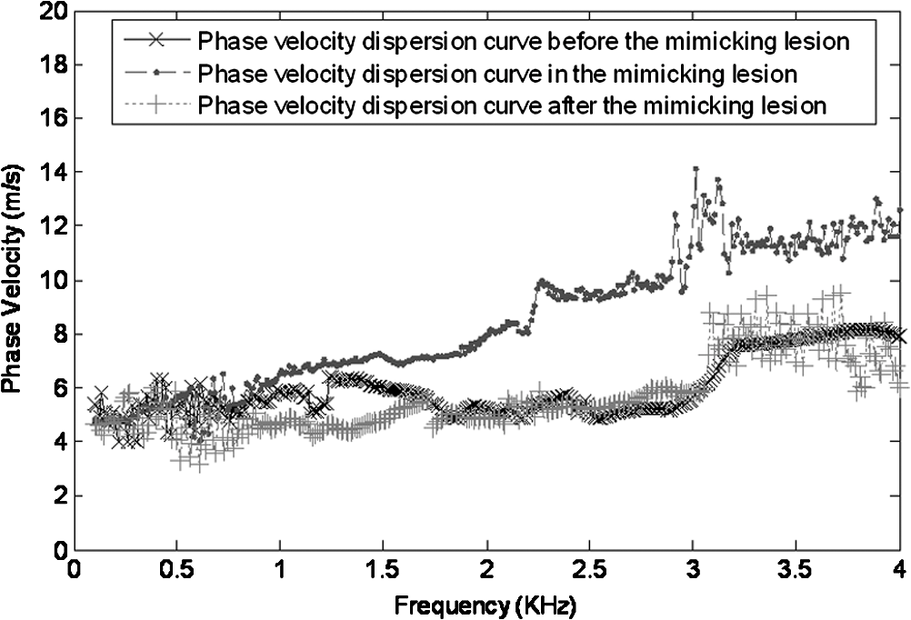
1.

Introduction

The alteration of biomechanical property of tissue is common in many tissue pathologies, such as skin conditions. Thus, assessing skin biomechanical properties is useful in improving our understanding of skin patho-physiology, which may aid medical diagnosis and treatment of, for example, skin cancer.^1–3 The prognosis of most skin cancers is important, because treatment at their early stages can improve five-year survival rate and increase the chance for cure.^4,5 For example, malignant melanoma (MM) is the most dangerous skin cancer, accounting for the majority ($\sim 75\%$) of deaths. In its early stage, the lesion is often confined within the epidermis and dermis ($\sim 1\mathrm{mm}$ thickness), with relatively higher Young’s modulus than the normal skin tissue. A diagnosis at this stage can improve the survival rate up to 90% to 100%.⁶ However, if diagnosed at a later stage, the tumor would have already invaded subcutaneous fat with a drastic increase of stiffness and become fatal.^7–9 Thus, tissue geometry and stiffness are important parameters for the clinical prognosis of skin diseases. Currently in clinic, the diagnosis of skin diseases largely depends on visual assessment by a trained dermatologist; however, there are often conditions where there is a clinical need for quantitative information on the skin’s mechanical properties. To meet this requirement, a sensitive, nondestructive, and noninvasive method that is capable of assessing the skin’s mechanical properties is therefore needed.

A number of elastography technologies, including imaging, have been developed that are suitable for qualitative and quantitative assessment of tissue mechanical properties. The main idea in elastography is to use a sensitive device to quantify the mechanical disturbance induced directly or indirectly by a mechanical stimulation, such as compression, vibration, or acoustic radiation.¹⁰ Ultrasound elastography^11–13 and magnetic resonance (MR) elastography^14,15 are popular and relatively developed methods in the medical diagnostic arena that use either ultrasound or MR imaging to measure the passive tissue disturbances, from which the mechanical properties of tissue interest are obtained remotely. Despite their success in cardiology,^16–19 they are difficult to quantify the skin properties, largely because of their low spatial resolution, which is not sufficient to image small lesions in the thin skin layers.

Optical coherence tomography (OCT)^20,21 is a promising noninvasive imaging technique capable of providing microstructural information on the skin, which has been reported to investigate a number of skin conditions, including cancers.^22–26 Due to its high-resolution nature, OCT has recently been extended to evaluate the skin mechanical properties both qualitatively and quantitatively,^27–37 generically termed optical coherence elastography (OCE). The methods that are used in OCE to monitor the passive tissue deformation induced by an external stimulus include the speckle tracking^27–30 and the tissue Doppler approaches,^31–34 with the latter being an order of magnitude more sensitive to the small tissue deformation than the former. Kennedy and Sampson et al. were the first to apply OCE for in vivo characterization of normal and hydrated human skins, relying on the dynamic two-dimensional (2D) OCT images³⁵ and more recently on three-dimensional (3D) OCT images.³⁶ Liang and Boppart³⁷ introduced a method that uses OCE to measure a continuous wave (CW) excited by an external shaker, from which they were able to quantify the elastic properties of human skin in vivo. These prior OCE methods used the OCT system to measure the induced shear wave propagation within tissue, by which the biomechanical properties of normal skin and skin lesions are assessed through analyzing the relative tissue displacement or the velocity of the shear waves. The shear wave approach generally works well if the investigated tissue is mechanically homogeneous. However, it becomes problematic when the tissue is heterogeneous, (e.g., layered structures), which is often the case for in vivo examination of human skin that has typically three layered structures. In addition, these prior OCE methods have an inherent disadvantage, i.e., they are not able to assess the mechanical properties of tissue at a depth beyond the OCT imaging depth, which is typically less than 1.5 mm beneath the skin surface.

To mitigate the aforementioned problems, our group recently pioneered an approach that combines the phase-sensitive OCT (PhS-OCT) with the surface acoustic wave (SAW) method to evaluate the elastic properties of layered thick tissues.^38,39 To facilitate the discussion in this paper, we term this method SAW-OCE. In SAW-OCE, a PhS-OCT is used to measure the surface waves at the tissue surface that are generated by an impulse stimulus, either by the use of a pulsed laser³⁸ or a mechanical vibration shaker.³⁹ Unlike the prior OCE methods, in which the maximum sensing depth is determined by the OCT imaging depth, the sensing depth in SAW-OCE is determined by the frequency contents (or bandwidth) of the generated surface acoustic waves that are measured at the tissue surface by PhS-OCT. Because PhS-OCT is sensitive to tissue motion with a sensitivity as small as $\sim 50\mathrm{pm}$,⁴⁰ the proposed SAW-OCE is shown to be suitable for characterization of elastic properties of thick tissues ($>5\mathrm{mm}$) with good system sensitivity.^38,39 Previously, we have shown that SAW-OCE can be used to provide quantitative elasticity of single, double-layer soft tissue mimicking phantoms^38,39 and normal human skin in vivo.³⁹ However, the previous studies assumed that the tissue is layered structures, i.e., the elasticity is changed axially (or vertically) into the depth. This assumption is valid in most of cases, particularly when normal skin is concerned. However, in skin pathologies, the lateral change of biomechanical properties has to be considered. For example, at the early stage of MM, the tumor is at invasive radial growth phase (lateral growth phase) with a thickness of typically less than 1 mm.^41–43 At this phase, the individual tumor cells start to acquire invasive potential and begin to spread in the lateral direction, but not in the axial direction. MM can be completely removed if there is a means to effectively detect the tumor at this stage.⁴¹ Tenderness on lateral palpation is suggestive of MM, because the early-stage disease is often localized, meaning the elasticity alters at the boundary between the normal and the diseased skin. Thus, the study of lateral alteration of elasticity of skin and skin diseases can offer a great potential to detect and localize the margin of skin diseases.

This paper is thus designed to investigate whether the SAW method is feasible to monitor the lateral alternation of the elasticity with a long-term aim to use SAW-OCE to provide localized and quantitative mechanical properties of heterogeneous biological tissues. To achieve this goal, we purposely designed a number of mechanically heterogeneous phantoms and ex vivo chicken breast tissues to simulate the localized changes of mechanical properties within the tissue in this study. A homemade shaker is used as the impulse mechanical stimulation that generates the surface acoustic waves propagating at the surface of tissue. The generated surface waves are then detected by a PhS-OCT system, a system that also provides depth-resolved microstructure information of the interrogated sample to assist the elasticity evaluation of the heterogeneous tissue. Surface wave phase velocity curves are calculated to give the heterogeneous elasticity of the sample.

2.

Brief Theoretical Aspects

The use of surface acoustic waves to evaluate mechanical properties of materials has been extensively studied over the last decade in the field of acoustics for industrial applications. Here, we provide a brief background in order to facilitate our discussion in this paper. Interested audience should refer to the literature for details.^44–47 When a material is stimulated with a mechanical impulse, ultrasonic waves can be generated, which propagate within the material. Among these waves, the P-waves (compression waves) and S-waves (shear waves) travel within the material, while the surface waves (also called Rayleigh waves) travel along the surface of the material. The Rayleigh wave is most widely used to characterize the elastic property of the industrial material. The propagation of surface waves in a heterogeneous medium (i.e., layered materials) shows dispersive behavior,⁴⁵ i.e., the different frequency components have different phase velocities. The phase velocity at each frequency is dependent upon the elastic and geometric properties of the material at different depths.⁴⁵ In isotropic homogeneous material, the surface wave phase velocity can be approximated as follows:^46–48

The above analyses are only applicable to the layered materials, i.e., elasticity of each layer is homogeneous. However, in the realistic in vivo situation, the tissue would often exhibit the lateral heterogeneity. In this case, when the acoustic waves travel to the boundary between two materials, the acoustic energy is either reflected or transmitted depending, on the material acoustic impedances. The acoustic impedance is the product of material density and acoustic wave velocity. A greater difference in acoustic impedance results in a greater percentage of energy that is changed at the interface or boundary between one medium and another. When a wave travels from material 1 to material 2, the following is required:⁵²

3.

System Configuration and Sample Preparation

3.1.

Generation and Detection of SAW

The system setup used to generate and detect the SAW is shown in Fig. 1, and it has been described in detail previously.³⁹ Briefly, the surface acoustic waves were induced by mechanical impulse stimulation from a homemade shaker. The shaker consisted of a signal generator and a single element piezoelectric ceramic with a metal rod attached at the end (length of $\sim 20\mathrm{mm}$ and diameter of $\sim 2\mathrm{mm}$) as a line source, which improved the signal-to-noise ratio (SNR) and enhanced the detection of the SAW compared with a point source.^53–55 A $\sim 20\mathrm{Hz}$ pulse train with a $\sim 0.2\%$ duty cycle was generated by the shaker, which produced frequency contents of up to $\sim 10\mathrm{KHz}$ in the SAW signals at the tissue surface. The detection of the shaker-induced SAW was accomplished by a PhS-OCT system. The PhS-OCT system employed a superluminecent diode as the light source, with a center wavelength of $\sim \mathrm{1,310}\mathrm{nm}$ and a bandwidth of $\sim 46\mathrm{nm}$, implemented by a spectral domain configuration.^56,57 And a 633 nm laser diode was used for aiming purposes during detection. The sample arm used an objective lens of $\sim 50\mathrm{mm}$ focal length to deliver the detection light on the tissue surface that coupled the SAW into the PhS-OCT for detection. The acquisition rate was determined by the spectrometer employed in the system that had a maximum rate of$\sim \mathrm{47,000}$ A-scans per second. For SAW detection, the system was configured as M-mode acquisition, while the OCT probe beam moved at the different locations on the sample surface. At the each location, 2,048 A-scans were acquired to obtain one M-mode scan, from which the phase changes due to the SAWs on the sample surface were evaluated. SAW displacements were calculated using:

Eq. (5)

$$\mathrm{\Delta }z=\frac{\mathrm{\Delta }\varphi \lambda }{4\pi n},$$

where $\mathrm{\Delta }\phi$ is the detected phase change, $\lambda$ is the central wavelength of the PR-OCT system (1,310 nm), and $n$ is the index of refraction of the sample ($\sim 1.35$). In the experiment, the average amplitude of generated SAW was typically $\sim 20$ to 30 nm. The total acquiring time of 43.5 ms was long enough and allowed the system to obtain one surface wave signal completely.

Fig. 1

Diagram of system setup of generation and detection of SAWs.

The OCT system also provided the microstructural images of the sample as a function of depth, i.e., the thickness of each layer, which allowed imaging of the layered tissue structures as well as the elastic properties of the tissue simultaneously. A trigger signal was given to both the shaker and the PhS-OCT system in order to fulfill the time-axial synchronization of the surface wave signals at each detected location on the sample surface. During the experiment, we moved the PhS-OCT sample beam to each detecting location while maintaining the shaker head at a fixed position pressing on the sample surface.

The signal processing procedure to obtain the phase velocity of SAW signals was similar to that in our previous publications.^38,39 Briefly, the signal’s noise was first minimized by the use of a Hilbert-Huang method that reduces the high-frequency random noise.⁵⁸ We calculated phase velocity dispersion curves of the SAWs detected at two adjacent positions. When the propagation wave has a wavelength equal to the travel distance $x1-x2$, the measured phase difference is $2\pi$. In general, the ratio between the phase difference and $2\pi$ equals the ratio of the distance to the wavelength:

Eq. (6)

$$\mathrm{\Delta }\phi /2\pi =(x1-x2)/\lambda ,$$

where $\mathrm{\Delta }\phi$ is the phase difference between two SAW signals at the locations $x1$ and $x2$. This can be calculated from the cross-power spectrum of two SAWs. In this way, the phase velocity ($V$) of the SAW traveling from $x1$ to $x2$ can be expressed as:

Eq. (7)

$$V=(x1-x2)\cdot 2\pi \cdot f/\mathrm{\Delta }\phi \mathrm{.}$$

Both the cross-power spectrum and the phase velocity dispersion curves are the key parameters for our analyses, as the former provides the available frequency range of the signals, while the latter gives the elastic and structural information of the sample. The cutoff frequency for the surface wave analysis was defined at $-20\mathrm{dB}$ from the maximum of the autocorrelation spectrum.^39,50 The final phase velocity dispersion curve was determined by averaging all the phase velocities between two detection points.

3.2.

Sample Preparation

As discussed in the introduction section, it is important to study the behavior of SAW traveling through the interface (boundary) at which the alternation of elastic property occurs, so that we could assess the feasibility of SAW-OCE to detect the localized change of elasticity within a mechanically heterogeneous tissue. Working toward this objective, we prepared three kinds of tissue phantoms (shown in Fig. 2) to simulate the localized change of elasticity, i.e., the alternation of mechanical property in both the lateral and axial directions.

Fig. 2

Schematic diagrams of three phantom models, showing the arrangement of the mechanical heterogeneity in phantoms.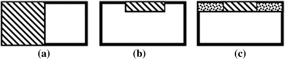

For phantom model-I [Fig. 2(a)], we intended to study the behavior of a surface wave when it travels across an interface between two materials with different elasticities. It is known that the higher the agar concentration, the higher the Young’s modulus of the gel becomes. Thus, we made two homogenous agar-gel blocks, one with a concentration of $\sim 1\%$ and the other of $\sim 3\%$. We then put them firmly together side by side to make the final phantom [Fig. 2(a), model-I] used in this study.

The skin lesion is often a localized inclusion with differing stiffness, which invades the normal epidermis and dermis; thus, in model-II [Fig. 2(b)], the phantoms were made to test the sensitivity of the surface wave method to the lateral changes in elasticity. We simplified the skin tissue with homogenous and soft chicken breast tissue, on to which a small but thin layer of stiffer mimicking-lesion near the surface was included. To accomplish this, we removed a part of tissue with a size of approximately $10\times 10\times 2(x,y,z){\mathrm{mm}}^3$ away from the bulk tissue, into which we implanted $\sim 3.5\%$ agar-gel. In another phantom, instead of using the stiffer agar-gel, we simply used a piece of the same breast tissue to fill the tissue volume that had been removed. This was because the procedures of making phantoms in the chicken breast tissue would inevitably leave a boundary behind at the interface between the bulk tissue and the lesion-mimicking tissue. Thus, this second phantom in this model would enable us to test whether the results obtained are influenced by the existing boundary in the phantom due to the phantom-making.

Skin is layered biological tissue, implying that the elasticity is altered along the depth, i.e., axially. Thus, in model-III [Fig. 2(c)], we incorporated the layered structures (two layers) into the model-II phantom in order to simulate skin that has a localized lesion, i.e., the elasticity is altered both axially and laterally. Because it was relatively challenging to make such a phantom using chicken tissue, we opted for the agar-gel in this case. The bulk phantom was made with $\sim 1\%$ agar as the base to mimic the subcutaneous fat tissue layer, on the top of which a $\sim 1.5\mathrm{mm}$ thick $\sim 2\%$ agar-gel was laid to simulate the dermis layer. And then, a $\sim 3.5\%$ agar-gel with a size of approximately $8\times 8\times 1.5{\mathrm{mm}}^3$ was implanted in the middle region to make the final phantom [see Fig. 2(c), model-III].

All the phantoms had a minimum thickness of $\sim 10\mathrm{mm}$, making the treatment of our measurements under the semi-infinite conditions valid. To improve the quality of OCT images to assist the assessment of elasticity, several drops of milk were mixed with the agar solution to increase scattering coefficient.

4.

Experimental Results

Figure 3(a) and 3(b) shows the typical surface waves recorded from the model-I phantom [Fig. 2(a)]. Figure 3(a) plotted the surface waves traveling across the interface (boundary) from stiff to soft tissue while the stimulation was located at the 3% agar-gel site, whereas Fig. 3(b) plotted the results while the stimulation was located at the 1% agar-gel site. The SAW-OCE sampled the surface waves first at the position about 2 mm away from the shaker head and then sequentially stepped to the required positions, with a step size of 1 mm, until 13 mm away from the shaker head. It is clear that the surface wave was moving away from the excitation position because the arrival time of the surface wave was increasingly longer when the detector was located farther away. The diamond sign marked the surface wave signal when it was passing through the interface between the two materials with different stiffness. Since it was a single-layer and homogeneous phantom at both sides of the sample, no velocity dispersion was found in the waveforms.

Fig. 3

Surface wave signal measured when it travels across an interface between two materials for the model-I phantoms: (a) from 3% to 1% agar side, while the excitation is located at the 3% site; and (b) from 1% to 3% agar side, while the excitation is located at the 1% site. The signal was measured initially at 2 mm position away from the excitation (bottom curve), and then sequentially stepped with 1 mm step size until 13 mm away from the excitation (top curve). Each curve is purposely shifted vertically by equal distance in order to better illustrate the results captured at different positions. The horizontal dotted lines indicate the baseline. The diamond marks the interface position. The same also applies to Figs. 5 and 9.

When the SAW travels across the interface from stiff to soft tissue [Fig. 3(a)], the wave speed in the 3% agar phantom ($\sim 11.58\mathrm{m}/\mathrm{s}$, evaluated from the diagonal line shown in Fig. 3) immediately dropped to the speed ($\sim 4.75\mathrm{m}/\mathrm{s}$) as if the SAW was traveling in the 1% agar-gel. In addition, the SAW amplitude was amplified at the interface (marked by diamond). On the contrary, in Fig. 3(b), the wave velocity increased (from $\sim 4.66\mathrm{m}/\mathrm{s}$ in 1% agar to $\sim 12.06\mathrm{m}/\mathrm{s}$ in 3% agar), but the SAW amplitude greatly attenuated at the interface. The measured SAW phase velocities in the 1% and 3% agar-gel sides in the model-I phantoms were matched well with those measured from the mechanically homogeneous single-layer phantoms reported previously.^38,39

To confirm the experimental results, we conducted a separate simulation by the use of finite-element (FEM) modeling, in which all the geometrical and physical parameters used in the experiments were plugged into the FEM program to obtain the numerical results. Please refer to the literature^59–61 for FEM modeling details. The simulated results of the SAW amplitudes are given in Fig. 4, along with those from the experiments for comparison. In addition, the experimental results obtained from the single-layer and mechanically homogeneous agar-gels (for 3% and 1% agar, respectively) are also shown in Fig. 4 to facilitate the comparison. From Fig. 4, we can observe that, for the mechanically homogeneous phantom of either 3% or 1% agar-gel, the SAW amplitude follows approximately an exponential attenuation when it travels away from the origin. For the model-I phantom, the SAW amplitude initially follows that from the homogeneous phantom until the SAW arrives at the interface. After the SAW crosses the interface, its amplitude is increased by $\sim 150\%$ when traveling from the 1% agar side to the 3% agar side [Fig. 4(a)]. In contrast, the SAW amplitude is decreased by $\sim 50\%$ when traveling in the opposite direction [Fig. 4(b)]. Both the experimental and FEM simulation results matched well with the theoretical expectations by Eq. (4), which indicates that the wave amplitude would increase by $\sim 150\%$ when passing through the interface from 3% agar to 1% agar and drop by $\sim 50\%$ when crossing the interface from 1% agar to 3% agar. Note here that in the theoretical estimation using Eq. (4), we estimated the necessary parameters based on the prior literatures:^38,39,62 the SAW velocity of 1% agar was $5\mathrm{m}/\mathrm{s}$, and that of 3% agar was $12\mathrm{m}/\mathrm{s}$; and the density of 1% and 3% agar-gel were $\mathrm{1,020}\mathrm{kg}·{\mathrm{m}}^3$ and $\mathrm{1,060}\mathrm{kg}·{\mathrm{m}}^3$, respectively. Note also that when traveling from the stiff side to the soft side, the SAW amplitude did not increase to its maximum immediately in the experiments [see Fig. 4(a)]. This was most likely due to the localization error during the experiments in which the interface was judged visually.

Fig. 4

The SAW amplitude evaluated from the experiments and FEM simulations. (a) surface wave travels from 3% agar to 1% agar and (b) surface wave travel from 1% agar to 3% agar. The diamond marks indicate the interface position.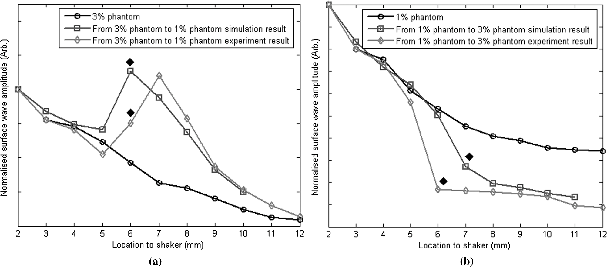

These results demonstrate that SAW-OCE is sensitive to the lateral change of elasticity in tissues, as measured by either the SAW velocity or the SAW amplitude. When crossing the boundary between two materials with differing elasticity, the SAW traveling speed would immediately adapt to that of the material it propagates. And more importantly, the observed abrupt change of the SAW amplitude can be taken as a marker to indicate that the SAW has traveled from one material to another and tell the relative location of material interface to the shaker, serving a potentially useful purpose in biomedical diagnosis.

Next, we used the model-II phantoms to analyse the sensitivity of SAW-OCE to a localized lateral alternation of elasticity. In order to make sure the enclosure of the localized stiffer material near the surface of the bulk chicken tissue, we first used the imaging mode of the PhS-OCT system to acquire cross-sectional microstructures images (B-scan) of the phantoms, immediately before the SAW experiments. Figure 5(a) shows the typical OCT image scanned from the phantom with the chicken breast tissue as the base and with 3.5% agar-gel as the localized stiffer inclusion to simulate a skin lesion, where the area “A” indicates the 3.5% agar-gel inclusion and the area “B” indicates the chicken breast tissue. The OCT image clearly demarcates the mimicked skin lesion that measured $\sim 10\times 1.8{\mathrm{mm}}^2$ in size ($\text{width}\times \text{depth}$). Figure 5(b) shows the typical OCT image obtained from another phantom made from the chicken breast tissue (area B) as the base with a small inclusion of the same tissue (area A) near the surface. As mentioned in the prior section, the second sample was made to check whether the existing boundary has an impact on the measured SAW results. In what follows, in order to facilitate the discussion, we call the phantom shown in Fig. 5(a) and 5(b) the Model-IIa and Model-IIb phantoms.

Fig. 5

Typical OCT image of the model-II phantom made from the chicken breast tissue. (a) chicken breast tissue as the base and a 3% agar-gel as the inclusion with a differing elasticity; where “A” indicates the agar inclusion and “B” the chicken breast tissue; and (b) chicken breast tissue as the base and another small but the same tissue as the inclusion near the surface, where “A” shows the localized inclusion and “B” the base tissue.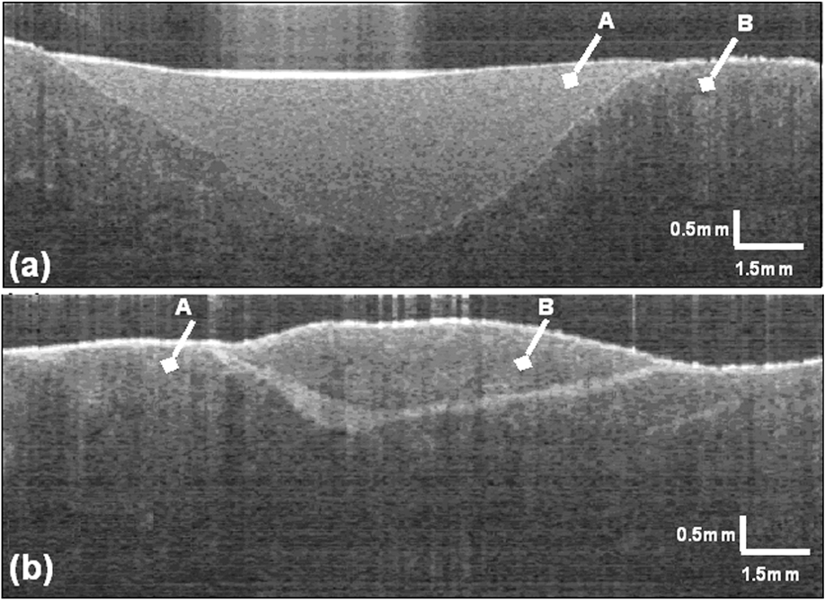

Figure 6(a) and 6(b) shows the typical surface waves measured from the Model-IIa and Model-IIb phantoms, respectively. The detection points were 1 mm adjacent apart, starting from the location at 2 mm away from the excitation and finishing at the location 13 mm away from the excitation. The distance spanned covered the interface between ex vivo chicken breast and mimicking lesion. From Fig. 6(a), we can observe that the surface wave began to disperse after it crossed the interface between chicken and agar, indicating that the SAW was traveling in a heterogeneous medium. On the other hand, there was no dispersion observed for the chicken-chicken sample [Fig. 6(b), Model-IIb], indicating the sample was a homogeneous material. The changes of SAW amplitude when traveling at the surface of the phantom were plotted in Fig. 7, from which a significant attenuation was observed when the SAW traveled across the boundary between chicken and 3% agar in the Model-IIa phantom. Assuming the chicken tissue and agar-gel used in this study have similar mass density (which is valid in our current study), the above result implies that the SAW velocity of 3.5% agar was higher than that of chicken breast, indicating that 3.5% agar had higher Young’s modulus. On the contrary, when the surface wave passed through the interface of the chicken-chicken phantom (Model-IIb), no abnormal attenuation in SAW amplitude was observed, indicating that the phantom is almost mechanically homogeneous. In other words, the boundary exited in the Model-IIb phantom does not have an effect on the proposed system sensitivity to measure the SAW.

Fig. 6

Surface wave signal measured when it travels along (a) the model-II phantom and (b) the model-IIb phantom, respectively. The signal was measured initially at 2 mm position away from the excitation (bottom curve), and then sequentially stepped with 1 mm step size until 13 mm away from the excitation (top curve).

Fig. 7

Surface wave amplitudes measured when the SAW travels in the model-II phantoms. The dark diamond marks indicate the position of the interface.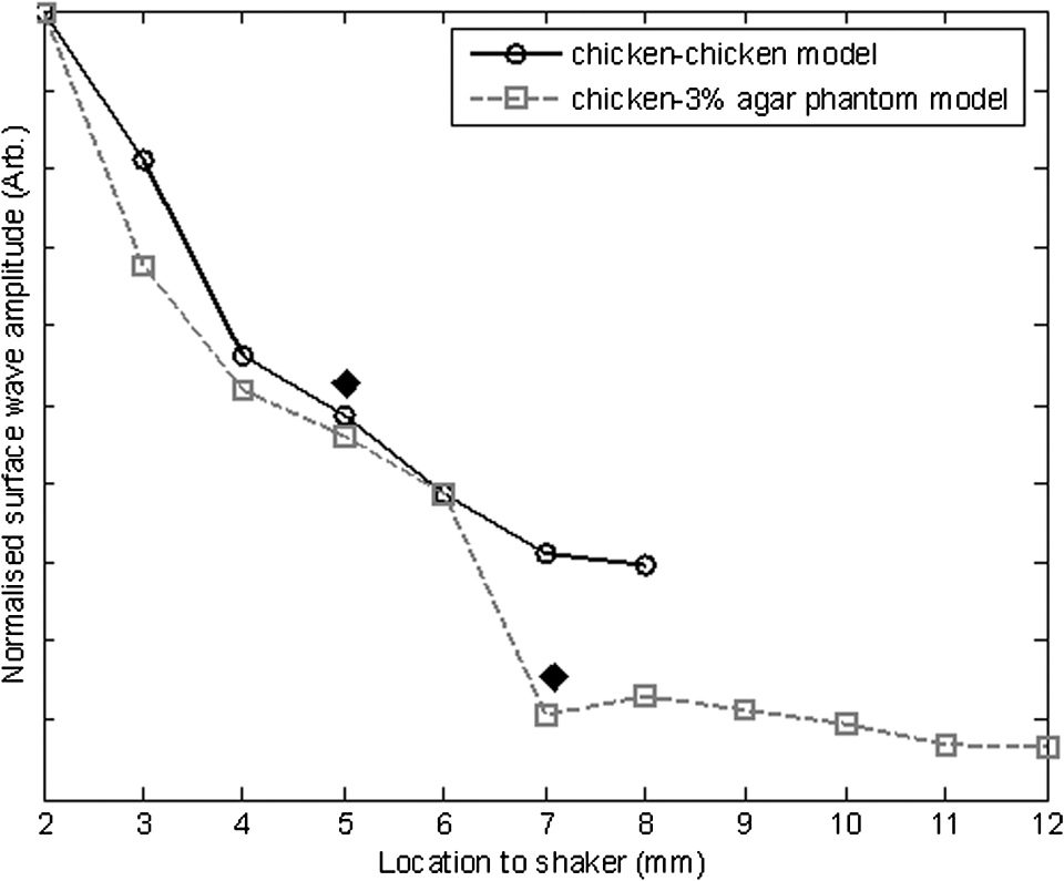

To further strengthen these observations and subsequent statements, we evaluated the SAW phase velocity curves from the measured signals. The results are illustrated in Fig. 8. The phase velocity curve of the SAW in the Model-IIb phantom (i.e., chicken-chicken sample) was almost a straight line ($\sim 7.19\mathrm{m}/\mathrm{s}$), asserting that the Model-IIb phantom was mechanically homogenous, at least under the current system sensitivity. The similar phase velocity curve ($\sim 6.89\mathrm{m}/\mathrm{s}$) was also observed for the Model-IIa phantom (i.e., chicken-3.5% agar sample), only before the SAW traveled into the mimicking lesion area. Note that a small difference in the low-frequency contents of these two curves might be caused by the dehydration of the chicken sample, as we used the same piece of chicken for these two experiments. However, the calculated phase velocity was increased after the SAW crossed the interface of chicken and 3.5% agar, showing the material was no longer mechanically homogenous. Here, the phase velocity ($\sim 7.08\mathrm{m}/\mathrm{s}$) in the low-frequency content (below $\sim 3\mathrm{KHz}$) represents the substrate chicken tissue, whereas the phase velocity ($\sim 13.13\mathrm{m}/\mathrm{s}$) in the high-frequency content represents the $\sim 3.5\%$ agar mimicking lesion, giving the Young’s modulus of $\sim 196\mathrm{KPa}$ and $\sim 595\mathrm{KPa}$, respectively. The Young’s modulus was calculated by using Eq. (1) by assuming the Passion’s ratio of $\sim 0.47$ and the density of $\sim \mathrm{1,060}\mathrm{kg}·{\mathrm{m}}^3$ for the $\sim 3\%$ agar,³⁹ and $\sim 0.49$ and $\sim \mathrm{1,060}\mathrm{kg}·{\mathrm{m}}^3$ for the chicken breast tissue, respectively.⁶² The evaluated elasticity values agreed well with the expectations drawn from the SAW amplitude measurements shown in Fig. 7. In addition, we were taught by Eq. (3) that the phase velocity curve can be used to estimate the thickness of the lesion. In this case, the calculated lesion depth of $\sim 1.96\mathrm{mm}$ agreed well with that measured from OCT images ($\sim 1.8\mathrm{mm}$). Note that the lateral resolution is determined by the distance between adjacent measuring points, which was 1 mm in the current study. This would ultimately limit the ability of the proposed method to accurately identify the border between two regions with different mechanical properties. Further study is warranted to determine the best lateral resolution that this approach can offer.

Fig. 8

Comparison of phase velocity dispersion curves between SAWs before and within the mimicking lesion for the model-II phantoms.

The experiments with the model-II phantoms demonstrate that SAW-OCE is sensitive to the thin layer of lateral alternations in elasticity. It is clearly possible that the SAW amplitude diagram can be used to locate the material interface, while the SAW phase velocity curve can be used to provide the elasticity information of different layers, as well as the thickness information about the inclusion with differing elasticity. In addition, we showed that the existing boundary between two materials with the same elasticity would not have an impact on the estimations of both the SAW amplitude and the phase velocity. However, the skin is a layered structure, so it is necessary to incorporate the layered features into the model-II phantom so that the sensitivity of SAW method to both the lateral and vertical elasticity changes can be assessed. The following study with the model-III phantom was designed to achieve this goal.

Figure 9 gives the typical OCT images acquired from the model-III phantom, which was made with $\sim 1\%$ agar as the substrate layer (area “C,” mimicking the subcutaneous fat), $\sim 2\%$ as the upper layer (area “A,” mimicking the dermis) and an $\sim 3\%$ agar inclusion ($8\times 1.3{\mathrm{mm}}^2$; $\text{width}\times \text{thickness}$) (area B, mimicking a skin lesion). Figure 10 shows the typical surface wave curves measured from this sample. The detection points were started at the location 2 mm away from the excitation, stepped across the sample with 1 mm increments, and finished at the position 19 mm away from the excitation, within which the whole inclusion was covered in the measurements. In this case, the system experienced two interfaces, one when stepped into and another out of the inclusion. Because this phantom had layered structures, the SAW dispersion was observed at all the measured locations as expected.

Fig. 9

Typical OCT B-scan image acquired from the model-III phantom, where “C” indicates the substrate layer (1% agar), “A” the upper layer ($\sim 2\%$ agar), and “B” the inclusion ($\sim 3\%$ agar), respectively.

Fig. 10

Surface wave signals measured from the model-III skin phantom starting at 2 mm (bottom in the left) and ending at 19 mm (top in the right) locations away from the excitation, with a 1 mm per step in between. The black diamonds marked the locations of the interfaces of the inclusion.

Figure 11 gives the extracted SAW amplitudes at all the measured positions, in which we can see that the SAW was greatly attenuated when it crossed the interface between $\sim 1\%$ agar and $\sim 3\%$ agar, and then increased when it traveled back into the $\sim 1\%$ agar. Both of the SAW waveforms and amplitude changes matched the width of the mimicking abnormal inclusion, as visualized and measured by the OCT B-frame images, demonstrating the feasibility of using SAW-OCE to localize the inclusion with a different elasticity from the substrate. This is important for developing this method into a diagnosing tool to differentiate diseased lesions from normal peripheral tissues.

Fig. 11

Surface wave amplitudes measured from the model-III phantom. The diamonds indicate the locations of the interfaces.

The evaluated SAW phase velocity curves before, within, and after the surface wave passed the mimicking lesion are provided in Fig. 12 for comparison, where we can clearly observe that the phase velocity curves before and after the SAW passed through the inclusion were similar to each other. The phase velocity values were evaluated to provide $\sim 4.79\mathrm{m}/\mathrm{s}$ in the low-frequency contents, which was increased to $7.5\mathrm{m}/\mathrm{s}$ at 3.2 kHz, representing the mechanical properties of the substrate layer and upper layer, respectively. The phase velocity curve for the SAW measured within the mimicking inclusion shared the similar surface waves in the low-frequency contents to the other measured locations, which is expected, because they all shared the same substrate layer. However, with the increase of frequency, the phase velocity began to represent the property of $\sim 3\%$ agar which was used to mimic the lesion layer, for which the phase velocity was evaluated at $\sim 12.08\mathrm{m}/\mathrm{s}$. The calculated thickness of the inclusion from the phase velocity curves was $\sim 1.4\mathrm{mm}$, which agreed well with that measured from the OCT B-frame images. Again, the phase velocity curve demonstrates the capability of the surface wave method to provide quantitative mechanical properties of a localized abnormal tissue, as well as to provide the geometrical thickness information.

Fig. 12

Comparison of phase velocity dispersion curves between surface waves when traveling in tissues before, within, and after passing the inclusion that mimics an abnormal lesion.

5.

Conclusion

We have presented a technique that combines a mechanical impulse induced SAW with a PhS-OCT system to detect and analyze the lateral alternations in mechanical properties of the mimicking lesion on the single and multi-layer mimicking agar phantoms and the ex vivo chicken breast tissue phantoms. We used a homemade shaker with a line shaker head to generate surface waves. Through the analyses of the SAW amplitude attenuations, it is clearly possible that the SAW method can be used to localize the interface between two materials with different elasticity properties. By analyzing the phase velocity curves evaluated from the detected surface wave signals, we have shown that the SAW is capable of providing and differentiating the elastic properties of a mimicking lesion from the normal peripheral tissues. In addition, the SAW method has also been shown to be useful in providing some important geometric information of the inclusions—for example, the thickness and the width, which agreed well with those determined by the use of the OCT imaging method. This study represents an important step toward the development of the SAW method as a clinical diagnosis tool to localize skin lesions and to quantify and differentiate the elastic properties of skin diseases from the normal surroundings.