Light-scattering flow cytometry for identification and characterization of blood microparticles

Anastasiya I. Konokhova; Maxim A. Yurkin; Alexander E. Moskalensky; Andrei V. Chernyshev; Valeri P. Maltsev; Elena D. Chikova; Galina A. Tsvetovskaya

doi:10.1117/1.JBO.17.5.057006

10 May 2012 Light-scattering flow cytometry for identification and characterization of blood microparticles

Anastasiya I. Konokhova, Maxim A. Yurkin, Alexander E. Moskalensky, Andrei V. Chernyshev, Valeri P. Maltsev, Elena D. Chikova, Galina A. Tsvetovskaya

Author Affiliations +

Journal of Biomedical Optics, Vol. 17, Issue 5, 057006 (May 2012). https://doi.org/10.1117/1.JBO.17.5.057006

Abstract

We describe a novel approach to study blood microparticles using the scanning flow cytometer, which measures light scattering patterns (LSPs) of individual particles. Starting from platelet-rich plasma, we separated spherical microparticles from non-spherical plasma constituents, such as platelets and cell debris, based on similarity of their LSP to that of sphere. This provides a label-free method for identification (detection) of microparticles, including those larger than 1 µm. Next, we rigorously characterized each measured particle, determining its size and refractive index including errors of these estimates. Finally, we employed a deconvolution algorithm to determine size and refractive index distributions of the whole population of microparticles, accounting for largely different reliability of individual measurements. Developed methods were tested on a blood sample of a healthy donor, resulting in good agreement with literature data. The only limitation of this approach is size detection limit, which is currently about 0.5 µm due to used laser wavelength of 0.66 µm.

1. Introduction

Blood microparticles are phospholipid vesicles derived from blood cell membranes. In particular, they are released from blood and endothelial cells during stress conditions, including cell activation and apoptosis.¹^,² These microparticles are relevant for many physiological processes, including intracellular crosstalk, transport, hemostasis, inflammation, and coagulation,³^,⁴ thus they are of scientific and clinical interest.

Both optical and non-optical methods are used for determination of microparticles size, morphology, concentration, biochemical composition, and cell of origin.⁵ One of the most popular methods for microparticles analysis is a flow cytometric assay. Flow cytometers of standard configurations provide measurement of the intensity of the light scattered in fixed range of angles, commonly forward (FSC) and side (SSC) scattering. That is not sufficient to distinguish large microparticles ( $\geq 1 μ m$ ) from platelets and aggregates of microparticles or small microparticles from electronic noise and cellular debris. Thus, microparticles size range is defined as 0.1–1 μm for commonly used cytometers. Flow cytometric protocols usually include microparticles isolation from blood sample through centrifugation to separate microparticles from platelets and particle size calibration using polystyrene microspheres of known size.⁶^,⁷ To distinguish microparticles from other blood particles or cellular debris, labeling with fluorescent markers is typically used.

Scanning flow cytometer (SFC) is capable of measuring angle-resolved light scattering pattern (LSP) of individual particles.⁸^,⁹ The LSP contains vast amount of information, which potentially can be used to deduce size, shape, and refractive index of individual particles.¹⁰^,¹¹ Fortunately, a homogeneous sphere is a good approximation to optical model of microparticles. For this simple model, a complete characterization (determination of size and refractive index) is possible by solving the inverse light-scattering problem.⁹^,¹² The only drawback is that the amplitude of the LSP rapidly decreases with size, resulting in a natural detection limit for any particle. The smallest reported size of polystyrene microspheres, processed with this method, is 0.6 μm,¹³ although sizes down to 0.2 µm can potentially be reached.¹⁴

In this paper, we develop a method to detect and characterize blood microparticles with the SFC. The method itself is developed in Sec. 2. It includes standard preparation of a platelet-rich plasma, measuring LSPs with the SFC, global optimization to find best-fit LSP, separation of blood microparticles from non-spherical blood constituents based on the similarity of its LSP to that of a sphere, a rigorous method to estimate errors of parameters estimates, and a procedure to estimate size and refractive index distributions over a sample. In Sec. 3, we illustrate the performance of a new method on a sample of blood from a healthy donor. Section 4 concludes the paper, discussing current limitations (e.g., in terms of detectable size) and directions for future research.

2. Materials and Methods

2.1.

Scanning Flow Cytometer

Technical features of the SFC and the operational function of the optical cell were previously described in detail elsewhere.⁹ The actual SFC fabricated by Cytonova Ltd. (Novosibirsk, Russia, http://cyto.kinetics.nsc.ru/) is equipped by 40 mW laser of 660 nm (LM-660-20-S) for generation of LSP of individual particles. Another 25 mW laser of 488 nm (Uniphase 2214-12SLAB) is used for generating trigger signal. The measured LSP is expressed as:⁹

Eq. (1)

I (θ) = \frac{1}{2 π} \int_{0}^{2 π} [S_{11} (θ, φ) + S_{14} (θ, φ)] d φ,

where

S_{i j}

are the elements of the

4 \times 4

Mueller matrix,¹⁵ and

θ

and

φ

are polar and azimuth scattering angles. In particular,

S_{11}

is the scattering intensity of unpolarized light. Moreover, for spherically symmetric scatterers,

S_{14} (θ, φ) \equiv 0

. The operational angular range of the SFC was determined from analysis of polystyrene microspheres, as described in Ref. 11, to be from 10-deg to 60-deg.

2.2.

Sample Preparation

Blood was taken from a healthy donor by venipuncture and collected in a vacuum tube containing ethylenediaminetetraacetic acid (EDTA) as anticoagulant ( $9 ∶ 1$ blood:EDTA). Within 1 hour of the collection, platelet plasma was obtained by centrifugation at 900 g for 15 min at room temperature. Polystyrene microspheres of sizes 1 and 2 µm (Molecular Probes, USA) were added for calibration of the SFC. The sample was 100-fold diluted in 0.22 µm filtered (FPV203030, Jet Biofil) 0.9% saline, and was analyzed with the SFC measuring the LSPs of all particles in the sample, including blood microparticles, platelets, 1 and 2 µm polystyrene microspheres and their aggregates, and cell debris. We plot all measured particles on a map of LSP integrated in angles from 10-deg to 60-deg versus LSP integrated in angles from 10-deg to 11-deg (Fig. 1). This is analogous to the $SSC \times FSC$ map used in conventional flow cytometers.¹⁶ Clusters corresponding to polystyrene microspheres and dimers of 1 µm microspheres are clearly visible—they define gates G1, G2, and G3. Based on them a broad gate, G4 is defined to include all potential events of microparticles. By definition, it also includes platelets and cell debris. It is important to note that no fluorescent labels were used to distinguish microparticles from other particles in gate G4; the LSP itself was used instead (see Sec. 2.4).

Fig. 1

Map of integrated LSP in angular range (10-deg, 60-deg) versus range (10-deg, 11-deg) in log-log scale for the whole sample. Polystyrene microspheres of 1 and 2 μm are gated by G1 and G3, respectively, while dimers of 1 μm polystyrene microspheres are gated by G2. Events in G4 (selected for further processing) include blood microparticles, platelets and cell debris.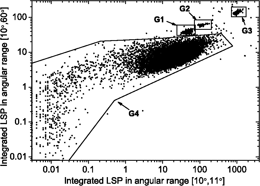

2.3.

Global Optimization

To solve the inverse light-scattering problem, we use a method previously developed in Ref. 11 for characterization of lymphocytes using the coated-sphere model. Here, we briefly describe this method. The problem is transformed into the global minimization of the weighted sum of squares:

Eq. (2)

S (β) = \sum_{i = 1}^{N} z_{i}^{2}, z_{i} = w (θ_{i}) [I_{th} (θ_{i}, β) - I_{\exp} (θ_{i})],

where

β

is a vector of two model parameters (sphere diameter

a

and refractive index

n

),

I_{th}

and

I_{\exp}

are theoretical and experimental LSP, respectively,

N = 512

number of LSP points (in the range of

θ

from 10-deg to 60-deg),

w (θ)

is weighting function to reduce an effect of the noise on the fitting results:¹¹

Eq. (3)

w (θ) = \frac{1 °}{θ} \exp [- 2 \ln^{2} (θ / 54 deg)] .

Theoretical LSPs for spheres are calculated using the Mie theory.¹⁵

To perform global optimization, DiRect algorithm was used.¹⁷ It provides an extensive search over the parameter space, described by rectangle $B$ , dividing it into a set of non-overlapping rectangles $V_{i}$ with centers $β_{i}$ , $i = 1, \dots, M$ . In addition to finding global minimum of $S (β)$ with the best estimate $β_{0}$ , it provides an approximate description of the whole surface of the minimized function by a set of values ${S (β_{i})}$ .¹¹ In our case, parameter space $B$ is confined by parameter bounds $a \in [0.1, 1.5] μ m$ , $n \in [1.34, 2.5]$ , which amply cover the range of blood microparticles.

2.4.

Identification of Blood Microparticles

The global optimization was applied to all particles in the gate G4. The next step is to discriminate blood microparticles from non-spherical particles, including platelets and cell debris.

All measured LSPs were fitted by the theoretical LSPs for spheres. Then we study the resulting residuals ${z_{i}}$ in detail. The general idea is that non-spherical particles should correspond to larger residuals than spherical. However, the absolute value of these residuals is not a completely rigorous measure, since additionally to shape it largely depends on size of the particle (data not shown). For a quantitative description of deviation from sphericity, we used two methods: Wald–Wolfowitz runs test¹⁸ and autocorrelation coefficient $ρ_{1} = \sum_{i = 2}^{n} z_{i} z_{i - 1} / \sum_{i = 1}^{n} z_{i}^{2}$ .¹⁹ However, we did not use Wald–Wolfowitz runs test in full. We only analyzed the number of runs $k$ , i.e. the number of sequences of adjacent deviations with equal (positive or negative) signs. It is also equal to the number of intersections of experimental and theoretical curves plus one. The number $k$ should tend to $N / 2 = 256$ for independent residuals, but is smaller when residuals are correlated. The coefficient $ρ_{1} \in [0, 1]$ is a direct measure of correlation between neighboring residuals.

A map of $k$ and $ρ_{1}$ for the gated sample G4 is shown in Fig. 2. One can clearly see two separate groups, which we identify as spherical and non-spherical particles, based on the following reasoning. For spherical particles the residuals are mostly caused by optical and electronic noise and imperfections of the optical system of the SFC. The latter may cause certain correlations between residuals, but they are expected to be minor. For non-spherical particles, the significant (or even major) source of residuals is model errors—the difference between the true LSP of the particle (without measurement noise) and the LSP of best-fit sphere. Since both these LSPs are smooth functions with almost no features, so is their difference, which implies small $k$ and large $ρ_{1}$ . The relation between measured LSPs and correlation measures is illustrated in Fig. 3, depicting typical spherical and non-spherical particles.

Fig. 2

Map of $ρ_{1}$ versus $k$ for a gated sample G4. The dashed line denotes threshold level for identification of blood microparticles ( 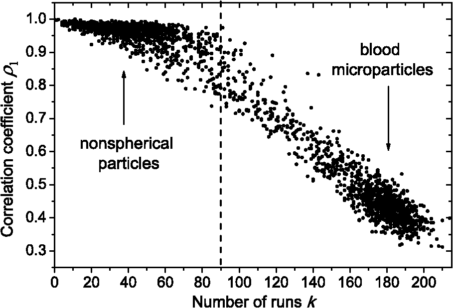$k > 90$ ).

Fig. 3

Results of global optimization for typical LSPs of (a) blood microparticle and (b) nonspherical particle, depicting weighted experimental and best-fit Mie theory LSPs. Best-fit value $β_{0}$ and correlation measures $k$ and $ρ_{1}$ are also shown.

It is possible to define a gate on the $k \times ρ_{1}$ map to identify blood microparticles; however, we chose a threshold for $k$ and (somewhat arbitrary) set its level to $k = 90$ . Finally, the blood microparticles were identified by condition $k > 90$ .

2.5.

Characterization of a Single Particle

While global optimization, described in Sec. 2.3, provides best-fit parameters $β_{0}$ for the measured LSP, a more detailed characterization is required including at least estimates of the parameters errors. Continuing along the lines of Ref. 11, we use the Bayesian approach to calculate probability density function $P (β)$ over parameter space for a given experimental LSP:

Eq. (4)

P (β) = κ {[S (β)]}^{- n_{eff} / 2}, κ = {\int_{B} [S (β)]^{- n_{eff} / 2} d β}^{- 1},

where

n_{eff} < N

is an effective number of degrees of freedom, which is used to approximately compensate for correlation between neighboring residuals, discussed in Sec. 2.4. It is determined by the structure of

I_{\exp} (θ) - I_{th} (θ, β_{0})

, see Ref. 11 for details. It is important to note that Eq. (4) implicitly assumes that prior probability distribution of

β

is uniform over

B

, which may potentially be corrected based on the dependence of LSP on

β

.¹⁹ Function

P (β)

provides a complete description of the information deduced from experimental LSP. In particular, one can calculate mathematical expectation of any quantity

f (β)

:

Eq. (5)

〈 f (β) 〉 = \int_{B} f (β) P (β) d β = \sum_{i = 1}^{M} f (β_{i}) P (β_{i}) V_{i},

where an integral is approximated by a discrete sum using the values

V_{i}

and

S (β_{i})

obtained during the execution of DiRect. According to Eq. (5), we calculate mathematical expectation

μ = 〈 β 〉

(generally different from

β_{0}

) and covariance matrix

C = 〈 (β - μ) {(β - μ)}^{T} 〉

. One can also obtain highest-posterior density (HPD) confidence regions with any confidence level

α

.¹¹

Since the procedure described in this section should be routinely applied to a large number of particles in a sample, it is not practical to store (and process) the complete set ${P (β_{i})}$ . A combination of $μ$ and $C$ can provide an adequate description of $P (β)$ if the latter is approximately equal to the density of bivariate normal distribution:

Eq. (6)

P_{N (μ, C)} (β) = \frac{1}{2 π \sqrt{\det C}} \exp {- \frac{1}{2} {(β - μ)}^{T} C^{- 1} (β - μ)} .

However, this should imply that

μ \approx β_{0}

and HPD confidence region is well described by ellipse

{(β - μ)}^{T} C^{- 1} (β - μ) = Q (χ_{2}^{2}, α)

. An example of processing a single experimental LSP [Fig. 4(a)] shows that these statements are far from being true. In particular, the HPD confidence region is bended.

Fig. 4

(a) HPD confidence region with confidence level $α = 0.95$ for size and refractive index of a single microparticle together with best-fit values $β_{0}$ , mathematical expectation $μ$ and approximate confidence ellipse based on covariance matrix. (b) The same but in auxiliary variables $u$ and $v$ . (c) Same as (a) but with mathematical expectation and confidence ellipse replaced by direct transformation of corresponding quantities from (b).

To understand this bending, we recall that for spheres with diameter much smaller than the wavelength the measured LSP is the following (Rayleigh scattering):¹⁵

Eq. (7)

I (θ) \sim a^{6} (\frac{m^{2} - 1}{m^{2} + 2}) (1 + \cos^{2} θ), m = \frac{n}{n_{0}}, n_{0} = 1.337,

where

n_{0}

is the refractive index of the medium. Even for spheres with sizes comparable to the wavelength, Eq. (7) describes the most significant part of dependence of LSP on

a

and

n

. In particular, the average bending of HPD confidence region in Fig. 4(a) can be described by

a y = const

, where

y = \sqrt[3]{(m^{2} - 1) / (m^{2} + 2)}

. To elaborate further on this correlation, we define two new dimensionless variables:

u = a y

and

v = y^{2} - a^{2} [γ = (u, v)]

, where

a

is assumed to be expressed in µm. The choice of

v

is somewhat arbitrary, the current simple choice makes the map

(a, y) \to γ

conformal, which, e.g., keeps orthogonality of coordinate grid during the mapping. However, the complete map

β \to γ

is not strictly conformal. The inverse map

γ \to β

is defined as follows:

Eq. (8)

a = \sqrt{\frac{\sqrt{v^{2} + 4 u^{2}} - v}{2}} μ m, n = n_{0} \sqrt{\frac{1 + 2 y^{3}}{1 - y^{3}}}, y = \sqrt{\frac{\sqrt{v^{2} + 4 u^{2}} + v}{2}} .

We repeat the same procedure to process experimental LSP, as described by Eqs. (2)–(5), but now in new variables

γ

. The only difference is that expression of

P (γ)

additionally contains non-trivial prior probability distribution of

γ

. The latter is equal to the Jacobian

| \partial β / \partial γ |

, which follows from uniform prior probability distribution of

β

. Therefore,

Eq. (9)

P (γ) = \tilde{κ} | \partial β / \partial γ | [{S (γ)]}^{- n_{eff} / 2}, \tilde{κ} = {(\int_{G} {[S (γ)]}^{- n_{eff} / 2} | \partial β / \partial γ | d γ)}^{- 1} \approx κ,

where region

G

is a rectangle:

u \in [0.01, 0.6]

and

v \in [- 2, 0]

, which approximately corresponds to

B

. For clarity, we define resulting mathematical expectation

ν = 〈 γ 〉

and covariance matrix

D = 〈 (γ - ν) {(γ - ν)}^{T} 〉

. Resulting HPD confidence regions are well described by ellipses and

ν \approx γ_{0} = argmin S (γ)

[Fig. 4(b)], so

P (γ)

is well described by a bivariate normal distribution, analogous to Eq. (6). This advantage can be easily illustrated in original variables as well [see Fig. 4(c)]. For example,

β (ν) \approx β_{0}

and point-by-point transform of the confidence ellipse approximates the original HPD confidence region, obtained in variables

β

. Moreover,

P (β)

is described by analytical expression

P (β) = P (γ) | \partial γ / \partial β |

. However, this is generally not required, since any integral over

P (β)

can be computed in

γ

-domain. For example, instead of Eq. (5) we obtain

Eq. (10)

〈 f (β) 〉 = \int_{B} f (β) P (β) d β = \int_{G} f [β (γ)] P (γ) d γ = \int_{G} \frac{f [β (γ)]}{2 π \sqrt{\det D}} \exp {- \frac{1}{2} {[γ - ν]}^{T} D^{- 1} [γ - ν]} d γ .

In particular, this can be used to calculate

μ

and

C

, but the results (data not shown) are almost the same as that obtained above in

β

-domain [see Fig. 4(a)].

Another simple way to characterize the particle is by projections of its HPD confidence region over each parameter, i.e. by the circumscribing rectangle: $[a_{\min,} a_{\max}] \times [n_{\min,} n_{\max}]$ . We name these as confidence interval although they are different from the commonly used marginal confidence intervals, defined through corresponding univariate probability distributions.

2.6.

Characterization of a Whole Sample

Each blood microparticle can be characterized with different levels of statistical description, ranging from best-fit values $β_{0}$ to a complete probability density function $P (β)$ . However, the final goal is to characterize the whole population of blood microparticles in a sample, e.g. by its distribution over size. The simplest way is to use only $β_{0}$ and plot it for all microparticles as a map [Fig. 5(b)] or as histograms (Fig. 6). The major drawback is that different values of $β_{0}$ have very different confidence levels, e.g. measured as errors of parameter estimates (Fig. 7), and hence should contribute differently to the total distribution. This mathematical problem consists in estimating the true distribution of parameters over the population in presence of (variable) measurement errors. To make this problem tractable, one has to make simplifying assumptions. For instance, in Ref. 11, multivariate normal distributions were assumed both for individual measurement errors and for distribution over sample. Then, parametric estimation of the latter is possible. The normality of distribution over sample seems justified for lymphocytes or other well-defined cell population, but, unfortunately, is not realistic for blood microparticles. First, blood microparticles originate from different sources¹ that may lead to multimodal distribution. Second, only part of the size distribution is sampled by the SFC due to the detection limit, which implies large asymmetry of the distribution.

Fig. 5

Map of best-fit parameters $β_{0}$ for (a) gated sample G4 and (b) separated subsample of blood microparticles.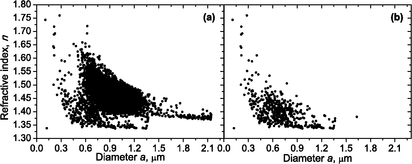

Fig. 6

Distributions of blood microparticles [same as in Fig. 5(b)] over best-fit parameters $β_{0}$ : (a) diameter and (b) refractive index.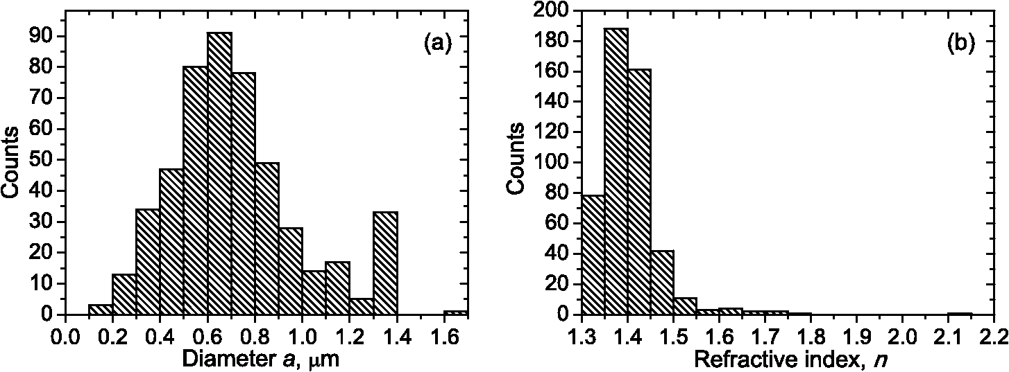

Fig. 7

Maps of standard deviation (in logarithmic scale) of (a) diameter and (b) refractive index versus its mathematical expectations $μ$ for blood microparticles.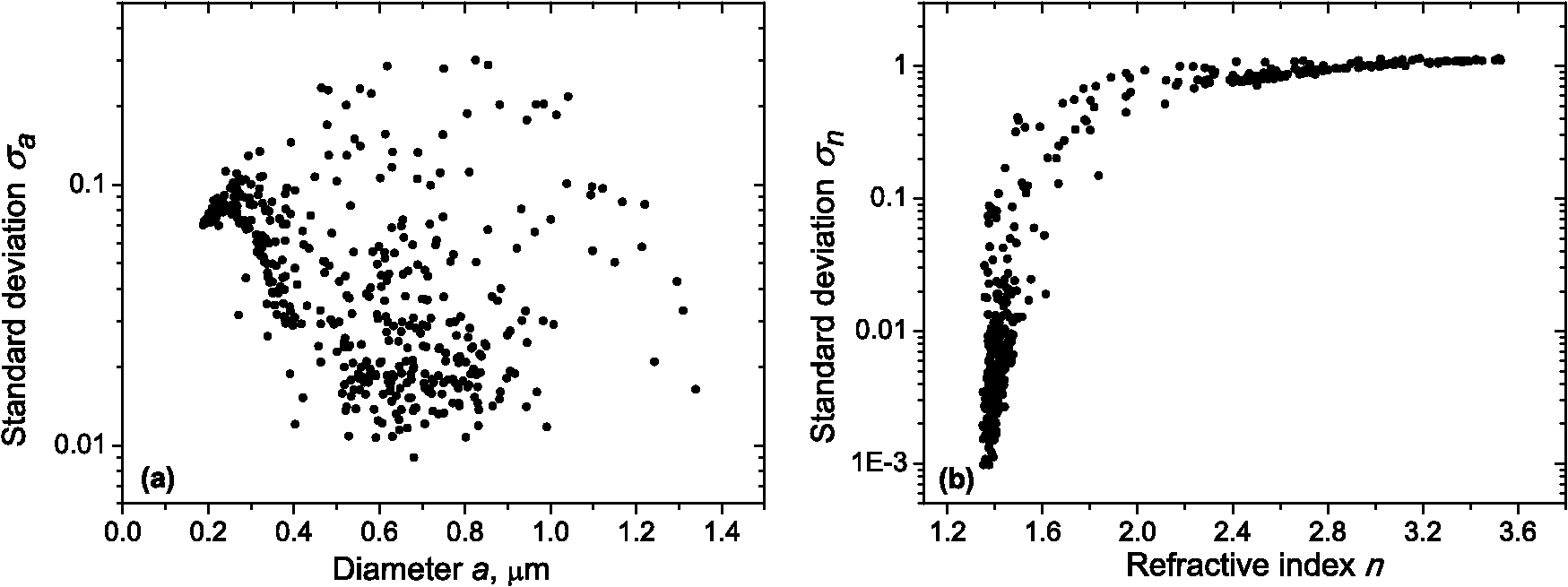

Since it is not feasible to use explicit parametric form for distributions over sample, we can only assume a certain smoothness of them. The corresponding problem is called deconvolution, which is significantly harder. To the best of our knowledge, in case of variable heteroscedastic measurement errors it has been solved only in univariate case with known density of these errors, either in analytical form (e.g. normal) or estimated from replicated data.²⁰ To solve deconvolution problem under this assumption we used the $R$ package decon.²¹ Limited by the method itself, we applied this package separately for size and refractive index. Moreover, we assumed normal marginal distributions for both parameters, which is reasonable if correlations are neglected anyway. Hence, for each parameter a set of values of mathematical expectation and standard deviation for each measured microparticle was given as input to the algorithm.

Also the results of deconvolution estimation strongly depend on the smoothing parameter—bandwidth (bw). To determine the optimal bandwidth, we applied the bootstrap-type method without resampling,²¹ implemented in the package decon to a part of experimental data with minimal errors: $σ_{a} < 0.1$ and $σ_{n} < 0.03$ , as shown in Fig. 8. The obtained values of bw, 0.0208 and 0.005 for $a$ and $n$ , respectively, were used for processing the whole dataset.

Fig. 8

Map of $σ_{n}$ versus $σ_{a}$ (both in logarithmic scale) for blood microparticles. A rectangle denotes particles that were used for calculation of the optimal smoothing parameter bw in the deconvolution algorithm.

Neglecting correlations between errors of size and refractive index is a rough approximation (Sec. 2.5), but at least this algorithm accounts for large difference of parameter errors between measured microparticles. Moreover, this algorithm allows processing all the particles in a single workflow, even those with very low quality of fit (huge errors in Fig. 8). This avoids use of arbitrarily-chosen threshold level required by alternative methods.

3. Results and Discussion

We measured LSPs of particles from the blood sample and defined the potential events of blood microparticles using the procedures described in Sec. 2.2. Additionally, we studied the negative control sample of 0.22 µm-filtered saline solution without platelet plasma—it contained only a minor amount of potential microparticles events (data not shown). Blood microparticles were separated from non-spherical blood constituents under the method described in Sec. 2.4. The power of this method is additionally exemplified by Fig. 5, which shows that neither best-fit values nor scattering integrals from Fig. 1 can differentiate blood microparticles from other plasma constituents.

The global optimization algorithm described in Secs. 2.3 and 2.5 was applied to each particle from the resulting subsample. Typical results of characterization of blood microparticles are shown in Fig. 9. Overall range of fit quality can be assessed by Figs. 7 and 8. Error of size estimates $σ_{a}$ increases with decreasing $a$ , which is due to decreasing signal-to-noise ratio, cf. Eq. (7).

Fig. 9

Typical results of characterization of blood microparticles. Estimates of particles parameters $μ$ , $σ$ , $β_{0}$ , and confidence intervals are also shown.

Characterization of the whole population of blood microparticles was performed according to Sec. 2.6. Resulting distributions over $a$ and $n$ are shown in Fig. 10. Comparing it with Fig. 6, we conclude that a rigorous deconvolution algorithm does make a difference and is required to produce reasonable results. However, the left wing of the size distribution [Fig. 10(a)] is evidently an artifact produced by the detection limit of the SFC. This limit strongly depends on $n$ , but below about 0.5 µm it leads to a bias in measured $n$ by discarding particles with smaller value of it [see Fig. 7(b)]. This size limit also corresponds to signal-to-noise ratio equal to 1 for $n = 1.39$ .

Fig. 10

Distributions of blood microparticles over (a) size and (b) refractive index, obtained using the deconvolution algorithm. Dashed line shows an estimate of current detection limit of the SFC.

Therefore, we indicate 0.5 µm by a dashed line in Fig. 10(a) as a limit of current version of the SFC. It is determined largely by the used wavelength (0.66 µm). Hence, decreasing it to 0.405 µm, as planned for the next version of the SFC, should allow accurate study of blood microparticles down to at least 0.3 µm. The fact that obtained size distributions start decreasing for larger value of $a$ (at about 0.7 µm) is due to the smoothness requirement used in deconvolution algorithm.

Our results for microparticles refractive index fall within the range typical for biological objects. Moreover, they are also similar to 1.39, which was used by other researchers for simulation of light-scattering properties of microparticles.⁵^,⁷ Overall shape of size distribution agrees in the range of [0.5,1] µm with other flow cytometric measurements, based on light scattering.⁷ or impedance²² measurements. However, these methods cannot reliably separate larger ( $> 1 μ m$ ) microparticles from platelets.

4. Conclusion

This paper describes a method for identification and characterization of blood microparticles using angle-resolved LSPs measured with the SFC. Label-free identification of blood microparticles, i.e. their separation from non-spherical constituents of platelet-rich plasma, was based on the structure of the LSP. In particular, number of intersections of experimental and best-fit theoretical LSPs were used, which has smaller values for non-spherical particles due to larger correlation between neighboring residuals. The identification method works for all microparticles, including those in the size range of platelets.

Each microparticle was characterized by fitting experimental LSPs with a homogeneous sphere model using the global optimization algorithm DiRect. Additionally to best-fit values of size and refractive index, we determined uncertainties (errors) of these parameters. The latter is described by standard deviations or alternatively by two-dimensional confidence regions. The latter is usually bended, which can be explained by dependence of light-scattering intensity on size and refractive index for small particles. To alleviate this issue, we introduced a change of model variables. Confidence region in new variables are well approximated by ellipses, thus allowing simple analytical description of confidence region in the original variables (size and refractive index).

To determine size and refractive index distributions of the whole population of microparticles, we applied state-of-the-art deconvolution algorithm, which accounts for largely different reliability of individual measurements. Unfortunately, this algorithm is limited to univariate data, thus we could not use all the information obtained at the characterization step. Accounting for correlation between uncertainties of size and refractive index during calculation of population distributions is left for the future research.

Developed methods were tested on a blood sample of a healthy donor, resulting in good agreement with literature data. The only limitation of this approach is size detection limit—currently, only microparticles larger than 0.5 µm are reliably processed. This limit is based on the laser wavelength of 0.66 µm. We plan to significantly decrease this limit by using shorter laser wavelength (e.g. 0.405 µm) and by overall improving of the SFC optical system to decrease signal-to-noise ratio.

Acknowledgments

This work was supported by grant from the program of Presidium of the Russian Academy of Science No. 2009-27-15, by the program of the Russian Government “Research and educational personnel of innovative Russia” (contracts P1039, P422, 14.740.11.0729, and 14.740.11.0921), by grant from Government of Russian Federation 11.G34.31.0034, and by the Program of the President of the Russian Federation for State Support of the Leading Scientific Schools (Grant NSh-65387.2010.4).

References

1.

L. Burnieret al., “Cell-derived microparticles in haemostasis and vascular medicine,” Thromb. Haemost., 101 (3), 439 –451 (2009). THHADQ 0340-6245 Google Scholar

2.

L. L. Horstmanet al., “New horizons in the analysis of circulating cell-derived microparticles,” Keio. J. Med., 53 (4), 210 –230 (2004). http://dx.doi.org/10.2302/kjm.53.210 KJMEA9 0022-9717 Google Scholar

3.

B. Hugelet al., “Membrane microparticles: two sides of the coin,” Physiology, 20 (1), 22 –27 (2005). http://dx.doi.org/10.1152/physiol.00029.2004 PHYSCI 1548-9213 Google Scholar

4.

A. PiccinW. G. MurphyO. P. Smith, “Circulating microparticles: pathophysiology and clinical implications,” Blood Rev., 21 (3), 157 –171 (2007). BLOREB Google Scholar

5.

E. Van der Polet al., “Optical and non-optical methods for detection and characterization of microparticles and exosomes,” J. Thromb. Haemost., 8 (12), 2596 –2607 (2010). http://dx.doi.org/10.1111/jth.2010.8.issue-12 JTHOA5 1538-7933 Google Scholar

6.

W. Jyet al., “Measuring circulating cell-derived microparticles,” J. Thromb. Haemost., 2 (10), 1842 –1843 (2004). http://dx.doi.org/10.1111/jth.2004.2.issue-10 JTHOA5 1538-7933 Google Scholar

7.

W. L. ChandlerW. YeungJ. F. Tait, “A new microparticle size calibration standard for use in measuring smaller microparticles using a new flow cytometer,” J. Thromb. Haemost., 9 (6), 1216 –1224 (2011). http://dx.doi.org/10.1111/j.1538-7836.2011.04283.x JTHOA5 1538-7933 Google Scholar

8.

V. P. Maltsev, “Scanning flow cytometry for individual particle analysis,” Rev. Sci. Instrum., 71 (1), 243 –255 (2000). http://dx.doi.org/10.1063/1.1150190 RSINAK 0034-6748 Google Scholar

9.

D. I. Strokotovet al., “Polarized light-scattering profile—advanced characterization of nonspherical particles with scanning flow cytometry,” Cytometry A, 79A (7), 570 –579 (2011). http://dx.doi.org/10.1002/cyto.a.v79a.7 1552-4922 Google Scholar

10.

V. P. MaltsevK. A. Semyanov, Characterisation of Bio-Particles from Light Scattering, VSP, Utrecht (2004). Google Scholar

11.

D. I. Strokotovet al., “Is there a difference between T- and B-lymphocyte morphology?,” J. Biomed. Opt., 14 (6), 1 –12 (2009). http://dx.doi.org/10.1117/1.3275471 JBOPFO 1083-3668 Google Scholar

12.

V. P. Maltsevet al., “Absolute real-time determination of size and refractive index of individual microspheres,” Meas. Sci. Technol., 8 (9), 1023 –1027 (1997). http://dx.doi.org/10.1088/0957-0233/8/9/011 MSTCEP 0957-0233 Google Scholar

13.

K. A. SemyanovV. P. Maltsev, “Analysis of sub-micron spherical particles using scanning flow cytometry,” Part. Part. Sys. Charact., 17 (5–6), 225 –229 (2000). http://dx.doi.org/10.1002/(ISSN)1521-4117 PPCHEZ 0934-0866 Google Scholar

14.

K. A. Semyanov, Google Scholar

15.

C. F. BohrenD. R. Huffman, Absorption and Scattering of Light by Small Particles, Wiley, New York (1983). Google Scholar

16.

R. NieuwlandA. Sturk, “Platelet-Derived Microparticles,” Platelets, 403 –413 Academic Press, USA (2007). Google Scholar

17.

D. R. JonesC. D. PerttunenB. E. Stuckman, “Lipschitzian optimization without the Lipschitz constant,” J. Optim. Theory Appl., 79 (1), 157 –181 (1993). http://dx.doi.org/10.1007/BF00941892 JOTABN 0022-3239 Google Scholar

18.

J. J. Higgins, An Introduction to Modern Nonparametric Statistics, Thomson Learning, Stamford, CT (2004). Google Scholar

19.

G. A. F. SeberC. J. Wild, Nonlinear Regression, Wiley-Interscience, Hoboken, NJ (2003). Google Scholar

20.

A. DelaigleA. Meister, “Density estimation with heteroscedastic errors,” Bernoulli, 14 (2), 562 –579 (2008). http://dx.doi.org/10.3150/08-BEJ121 1350-7265 Google Scholar

21.

X. -F. WangB. Wang, “Deconvolution estimation in measurement error models: the

R

package decon,” J. Stat. Software, 39 (10), 1 –24 (2011). 1548-7660 Google Scholar

22.

J. I. Zwickeret al., “Tumor-derived tissue factor-bearing microparticles are associated with venous thromboembolic events in malignancy,” Clin. Cancer Res., 15 (22), 6830 –6840 (2009). http://dx.doi.org/10.1158/1078-0432.CCR-09-0371 CCREF4 1078-0432 Google Scholar

Citation Download Citation

Anastasiya I. Konokhova, Maxim A. Yurkin, Alexander E. Moskalensky, Andrei V. Chernyshev, Valeri P. Maltsev, Elena D. Chikova, and Galina A. Tsvetovskaya "Light-scattering flow cytometry for identification and characterization of blood microparticles," Journal of Biomedical Optics 17(5), 057006 (10 May 2012). https://doi.org/10.1117/1.JBO.17.5.057006

Published: 10 May 2012

Access the abstract

JOURNAL ARTICLE
9 PAGES

DOWNLOAD PAPER SAVE TO MY LIBRARY

GET CITATION

CITATIONS

Cited by 48 scholarly publications and 3 patents.

Explore citations on Lens.org

RIGHTS & PERMISSIONS

Get copyright permission Get copyright permission on Copyright Marketplace

KEYWORDS

Blood

Particles

Refractive index

Error analysis

Flow cytometry

Optical spheres

Deconvolution

1.

Introduction

2.

Materials and Methods

2.1.

Scanning Flow Cytometer

Eq. (1)

2.2.

Sample Preparation

Fig. 1

2.3.

Global Optimization

Eq. (2)

Eq. (3)

2.4.

Identification of Blood Microparticles

Fig. 2

Fig. 3

2.5.

Characterization of a Single Particle

Eq. (4)

Eq. (5)

Eq. (6)

Fig. 4

Eq. (7)

Eq. (8)

Eq. (9)

Eq. (10)

2.6.

Characterization of a Whole Sample

Fig. 5

Fig. 6

Fig. 7

Fig. 8

3.

Results and Discussion

Fig. 9

Fig. 10

4.

Conclusion

Acknowledgments

References

Show All Keywords

Keywords/Phrases

Search In:

Publication Years