|
|
1.IntroductionThe majority of the image-reconstruction algorithms developed for photoacoustic tomography (PAT) or optoacoustic tomography (OAT) have assumed a lossless acoustic medium. The effect of frequency-dependent attenuation on acoustic waves can be significant, since the ultrasonic waves generated by pulsed lasers can be extremely broadband.1 Reconstructed images may exhibit distortion and artifacts if these effects are not taken into account. Several researchers have looked at the effect of acoustic attenuation in OAT. Previous work on dispersive acoustic media done by La Rivière et al.2 focused on incorporating the frequency-dependent attenuation effects into the OAT model. They related the attenuated pressure in a lossy medium to the ideal pressure in a lossless medium via an integral operator. More recently, several groups1,3–4.5 have used the time-reversal (TR) approach to address attenuation in PAT. This method is based on the use of an acoustic forward model in which the absorption operators are reversed in sign. Roitner and Burgholzer6 have looked at a complex frequency-approach regularization method to correct for acoustic attenuation in PAT. In this work, we will use an approach similar to that by Markel et al.,7,8 in optical-diffusion tomography, to derive an inversion formula for the absorbed optical absorption energy using singular-value decomposition (SVD). This formula is applicable in a planar detector geometry. It provides insight into the conditioning of the inverse problem and offers a promising method for image reconstruction in an attenuating medium. This expression directly relates the measured attenuated pressure to the absorbed optical energy. We also study the noise and resolution properties of this SVD-based algorithm. 2.Correction for Ultrasonic Attenuation in OAT Using SVD2.1.MethodsIn an attenuating medium, the optoacoustic wave equation includes a loss term2,9,10 and is given by: where and where is the temporal frequency, is the linear attenuation coefficient, is the complex wave number, is the measured pressure at point and time , is the coefficient of volume expansion, is the specific heat and is the speed of sound. is the heating function that denotes the energy deposited per unit time per unit volume by the illuminating optical pulse and is given by: where is the absorbed optical energy and is the temporal profile of the optical pulse.For soft biological tissue, the attenuation coefficient has a power-law dependence on the frequency given by:11 In tissues, typical values for ultrasonic attenuation are: and (Ref. 11).Using the Kramers-Kronig relations, for power-law absorption with and , one obtains the dependence of phase velocity on frequency due to frequency-dependent attenuation as:9 where is the speed of sound at a reference frequency of .For , the dependence of phase velocity on frequency due to frequency-dependent attenuation is given by: So for an attenuating medium, Eq. (1) becomes: where is the temporal Fourier transform of measured pressure and is the temporal Fourier transform of the illumination pulse.This equation can be solved using standard Green’s function methods as:12 where and is the Green’s function.2.1.1.Angular spectrum expansion of the measured pressure signalsThe angular spectrum expansion of the Green’s function is given by:13 Substitute this in Eq. (8) and consider the pressure measurements on the plane and we get:We assume that the photoacoustic object lies in the plane . On taking the Fourier transform on both sides and reducing the resulting expression, one obtains the angular spectrum expansion of measured photoacoustic pressure as: 2.1.2.SVD of integral operator relating pressure to optical-absorption coefficientWe follow Markel’s7,8 approach to optical-diffusion tomography to obtain an integral operator relating the measured attenuated pressure to the absorbed-optical-energy density. Define a two-dimensional (2-D) spatial wave vector as: We then discretize the temporal frequency, as . For notational simplicity, we use instead of in the following equations. One can then write the pressure as:where .Define , . Thus, one can obtain an integral equation: where This equation can be inverted as:8where the operator denotes the complex conjugate of matrix , and is the inverse of matrix .We can obtain a simpler expression for by performing the integral over . Equation (18) can be written as: where .This can be reduced to: Thus the desired image of the absorbed optical energy is obtained by: where is the 2-D spatial vector.The computation of the inverse of the matrix is the key step in the procedure to recover the absorbed optical energy. Its pseudoinverse can be computed by performing the SVD of the matrix . Some of the eigenvalues of this matrix may be zero or very small. One will need to use regularization to circumvent this problem. Thus, the procedure for recovering is:
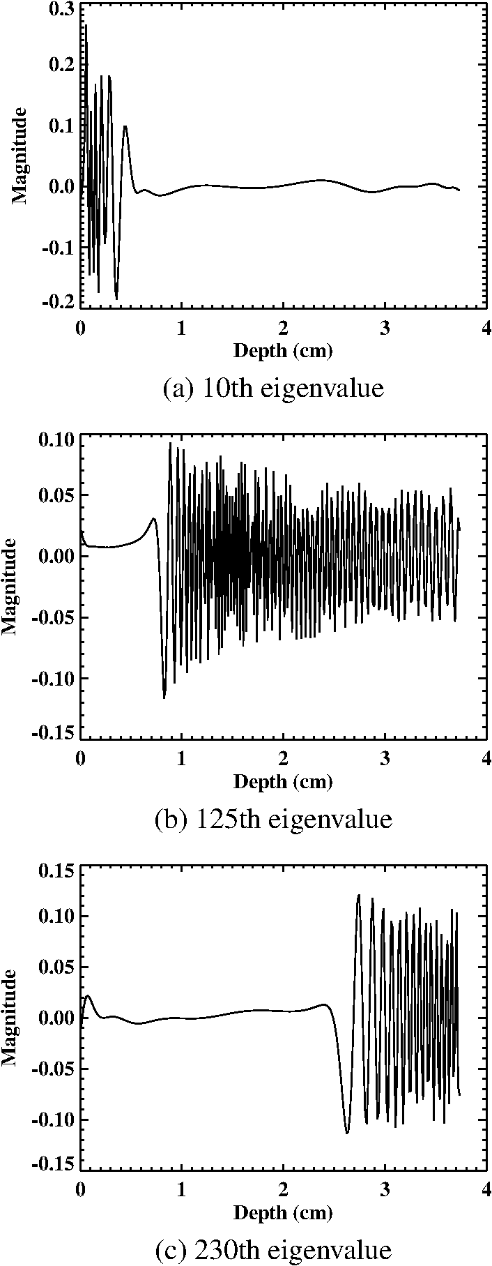
2.1.3.Calculation of eigenvalues of M matrix with nonzero attenuationTo investigate the posedness of the inverse problem we examined the properties of the matrix and its singular values for a medium with nonzero attenuation. We computed this matrix for a typical tissue with attenuation and . A set of 250 discrete temporal frequencies and 64 discrete spatial frequencies was used. Temporal frequencies ranged from 0 to 5 MHz and spatial frequencies ranged from 0 to . This corresponds to the transducer elements spaced 0.05 cm apart. We performed an SVD of the matrix . The eigenvalues of the matrix were obtained from the singular values of matrix . The variation of eigenvalues of for various spatial frequencies “” is shown in Fig. 1. Figure 2 shows the variation of the eigenvectors of matrix with depth for a specific eigenvalue. From these plots one concludes that:
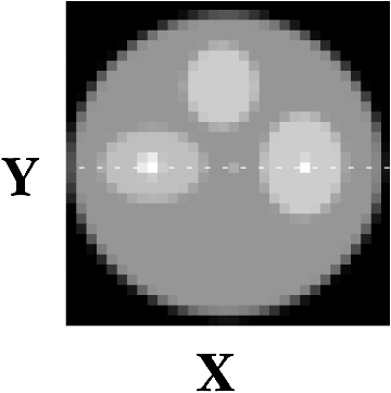
The behavior of eigenvectors and eigenvalues indicates that shallower objects can be recovered much better than deeper objects because they correspond to eigenvectors with much higher eigenvalues. We also observe that eigenvectors that correspond to smaller eigenvalues also have much higher frequency components. This implies that resolution will degrade as you go deeper and that the higher frequencies cannot be recovered as accurately. 2.2.Image-Reconstruction DetailsTo investigate the performance of the SVD-based algorithm, several reconstructions were performed. The sensor data was simulated using the k-Wave toolbox,14,15 which uses the k-space method13 to model the propagation of optoacoustic waves in lossy media. Both a point source placed at different depths and a three-dimensional (3-D) phantom were used to define the initial pressure distribution. For the point source, a grid size of voxels was used () supporting temporal frequencies up to 1.5 MHz. The temporal sampling interval was set to 100 ns and the simulations performed using 256 time steps. For the 3-D phantom, a grid size of voxels was used () with the same temporal sampling interval and 512 time steps. In both cases the sensor data was recorded in the plane , corresponding to sensor positions for the point-source simulations and sensor positions for the 3-D phantom. The attenuation coefficient was set to , a value of was used for the power-law frequency dependence, and the speed of sound was set to . For each investigated case, several reconstructions were performed. First, the SVD-based method was used by obtaining the inverse of the matrix using truncated SVD (as described in Sec. 2.1.2). The magnitude of the eigenvalues of for a specific was used to regularize the pseudoinverse of for that . For comparison, the images were also reconstructed using TR.1,5 The TR reconstructions were performed both with and without compensation for acoustic absorption. When absorption compensation was included, the reconstructions were regularized by filtering the absorption and dispersion terms within the governing equations using a Tukey window. This restricts the range of frequencies that are allowed to grow during the reconstruction. The filter cut-off frequency (which acts as the regularization parameter for the TR algorithm) was chosen by examining the spectrum of the recorded sensor data.5 To separate the effect of limited-view artifacts (which are common to all reconstruction algorithms for this sensor geometry), an ideal reconstruction was also generated using TR with the absorption parameters set to zero in both the forward and inverse problems. (This is referred to as the ideal-TR-based reconstruction in the following sections.) 3.Results3.1.Sensitivity of SVD-Based Reconstruction to Regularization ParameterWe found that the quality of the reconstructed images using our SVD-based method was very sensitive to the regularization parameter used. The resulting magnitude and sharpness of the reconstructed images varied with this parameter. We chose the regularization parameter to depend on and related it to a certain percentage of total eigenvalue energy at that . Specifically, the truncation parameter for a given matrix for a given was chosen to be: where . The eigenvalue energy, for a given , for eigenvalues was defined as: Figure 3 shows how the reconstructed SVD-based images for a point source, at two different depths, vary with . The regularization parameter that gives the best image also depends on the value of attenuation and how much noise is present in the data, and it has to be adjusted when noise level or attenuation changes.Fig. 3Variation of SVD-based images with the regularization parameter as a percentage of total energy of the eigenvalues. 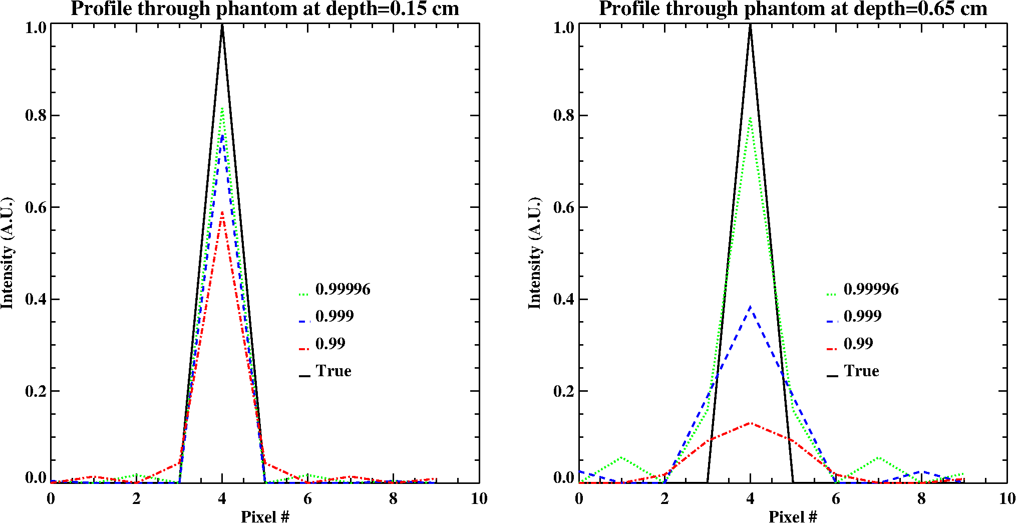 In general, there is no clear rule to help us decide what is a good value for the regularization parameter. It depends on how one evaluates image quality and what is the detection task. Image quality assessment depends both on the task and the observer,16 and a given technique may not perform well for all possible applications. One has to consider various image-quality aspects like spatial resolution, contrast, signal-to-noise ratio (SNR), artifacts, suppression of noise, signal detectability, quantitative accuracy, etc. We found that even in the absence of random noise in the data, we still had to use regularization as defined above to obtain a good-quality image that matches well with the true phantom. The need for regularization in this case may be arising from the very nature of the matrix , since it is exponentially damped. It could also arise from the effect of rounding and discretization errors. Further investigation is needed to understand and address this issue. 3.2.Noiseless DataIn the following results, a value of was used for the SVD-based images. All the images were reconstructed using attenuated-pressure data generated using the -Wave toolbox. The cropped reconstructed images using SVD-based reconstruction and the TR algorithm are shown below in Fig. 4. The reconstructed images using SVD bear a close resemblance to the ideal image. Fig. 4Reconstructed -slice at a depth of 0.25 cm of a 3-D phantom, left to right: true phantom, SVD-based image, ideal-TR-based image, corrected-TR-based image, uncorrected-TR-based image.  Figure 5 shows the line used for the y-profile shown in Fig. 6, in the slices and of the reconstructed for noiseless data. 3.3.Noisy DataRandom Gaussian noise was added to the attenuated-pressure data, generated using the -Wave toolbox, to obtain a SNR of 45 dB. A value of was used for regularization in the SVD-based method for the slice at 0.25-cm depth. A value of was used for regularization in the SVD-based method for the slice at 1.0 cm depth so as to reduce noise amplification. Figure 7 shows the cropped reconstructed phantom images using noisy attenuated pressure. Fig. 7Reconstructed -plane at a depth of 0.25 cm reconstructed using noisy attenuated pressure, left to right: true phantom, SVD-based image, ideal-TR-based image, corrected-TR-based image, uncorrected TR-based image.  Figure 8 shows the -profile along the line shown in Fig. 5, in the slices and of the reconstructed absorbed optical energy for noisy data. The reconstructed images based on the noisy simulatedpressures obtained via the SVD-based method are in good agreement with the ideal image. The SVD-based image-reconstruction algorithm offers comparable images even with noisy data, although it is more sensitive to the presence of noise. 3.4.Depth ResolutionFigure 9 shows the profile through a point source placed at various depths reconstructed using SVD-based attenuated pressure. The plot labeled “True” refers to the original point source. The label “TR-based” refers to corrected TR-based reconstructed image, while the label “Uncorrected TR-based” refers to uncorrected TR-based reconstructed image. Fig. 9Line profile of a point source placed at a depth of 0.15 and 0.65 cm for images reconstructed using: TR method corrected for attenuation, TR method, and SVD-based method.  Table 1 lists the full width at half maxima (FWHM) for the point-source images constructed using the different algorithms. Table 1FWHM in cm for a point-source image at different depths constructed using SVD-based and TR-based algorithms.
The SVD-based image reconstruction algorithm shows very good depth resolution, especially for depths up to 0.35 cm. At greater depths this algorithm offers worse resolution when compared to images reconstructed using the TR-based method with or without attenuation correction. However, the intensity of the image reconstructed using the SVD-method at greater depths relative to shallower depths is much higher than that obtained from the TR-based method with attenuation correction. As mentioned before, the depth resolution of the images reconstructed via the SVD-based method are also dependent on the choice of the regularization parameter. In practice, we may be able to attain better depth resolution using the SVD-based method by adjusting this parameter. 4.DiscussionOur SVD-based method provides insight into the ill-conditioning of the inverse problem of image reconstruction in PAT in a lossy medium. However, there are several important issues to consider in using this approach. One needs to address the choice of regularization method used to obtain the matrix inverse of matrix . We found that there was a need for regularization even in the absence of noise. We used a truncated SVD method for regularization. The truncation of eigenvalues was based on a certain percentage of total energy contained in all the eigenvalues. Our choice of this type of truncation was based on obtaining good resolution at greater depths. However, there are many other methods for regularizing, and there are several excellent references in the literature17 that address this issue extensively. A systematic study of the choice of regularization parameter for our SVD-based image-reconstruction method remains a subject for further study. Both the TR-based and the SVD-based image-reconstruction techniques use regularization to prevent high-frequency noise present in the sensor data being amplified during the reconstruction. However, there is a distinct difference between these techniques in how this regularization is applied. In the TR-based approach, the range of frequencies that is allowed to grow is restricted by filtering the absorption parameters within the governing equations. This restriction applies to signals originating from all depths within the medium. However, in practice, some of the high frequency components from shallow features within the image may be above the noise floor, while the same frequency components from deeper features may not. This method of regularization does not allow for the selective compensation of the attenuation at these frequencies. Conversely, in the SVD-based approach, the regularization is based on the magnitude of the eigenvalues where the corresponding eigenvectors have features at different depths. This allows for the compensation of the attenuation of high-frequency components originating from shallow features, even if the corresponding frequency components from deeper features are not above the noise floor. Finally, it is useful to note that, while the SVD-based method is computationally intensive, this may be justified in cases where the quantitative accuracy of the reconstructed pressure distribution is of importance. For example, in quantitative photoacoustics where the goal is to derive accurate chromophore concentrations,18 errors in the reconstructed pressure due to acoustic attenuation will ultimately result in errors in the extracted quantitative information. 5.ConclusionsWe derived an operator relating the attenuated pressure to the absorbed optical energy to reconstruct images in PAT in an attenuating medium for a planar geometry. We derived an SVD-based algorithm based on this operator to reconstruct the absorbed optical energy in PAT in an attenuating medium. We looked at the eigenvalues of the matrix which is used to recover the absorbed optical energy. We found that smaller values of the 2-D spatial frequency vector are recovered much better than the larger values. We also observed that the smaller eigenvalues typically corresponded to eigenvectors with most of their energy at greater depths. The behavior of eigenvectors and eigenvalues indicated that shallower objects can be recovered much better than deeper objects because they correspond to eigenvectors with much higher eigenvalues. The SVD-based approach to the attenuation problem in PAT offers a promising method for direct image reconstruction in a planar geometry. It also provides a way to study the conditioning of this inverse problem. This SVD-based algorithm shows good depth resolution and noise stability. However, we found that the image quality of the reconstructed images was very sensitive to the choice of regularization parameter used for obtaining the inverse of via SVD. AcknowledgmentsDimple Modgil would like to thank Mark A. Anastasio for helpful discussions related to this work. This work was supported in part by a breast cancer predoctoral research award (W81XWH-08-1-0331) to Dimple Modgil. ReferencesB. E. Treebyet al.,
“Acoustic attenuation compensation in photoacoustic tomography: application to high-resolution 3d imaging of vascular networks in mice,”
Proc. SPIE, 7899 78992Y
(2011). http://dx.doi.org/10.1117/12.874530 Google Scholar
P. J. La RivièreJ. ZhangM. A. Anastasio,
“Image reconstruction in optoacoustic tomography for dispersive acoustic media,”
Opt. Lett., 31
(6), 781
–783
(2006). http://dx.doi.org/10.1364/OL.31.000781 OPLEDP 0146-9592 Google Scholar
P. Burgholzeret al.,
“Compensation of acoustic attenuation for high-resolution photoacoustic imaging with line detectors,”
Proc. SPIE, 6437 643724
(2007). http://dx.doi.org/10.1117/12.700723 Google Scholar
P. Burgholzeret al.,
“Information changes and time reversal for diffusion-related periodic fields,”
Proc. SPIE, 7177 717723
(2009). http://dx.doi.org/10.1117/12.809074 Google Scholar
B. E. TreebyE. Z. ZhangB. T. Cox,
“Photoacoustic tomography in absorbing acoustic media using time reversal,”
Inv. Prob., 26
(11), 115003
(2010). http://dx.doi.org/10.1088/0266-5611/26/11/115003 INPEEY 0266-5611 Google Scholar
H. RoitnerP. Burgholzer,
“Efficient modeling and compensation of ultrasound attenuation losses in photoacoustic imaging,”
Inv. Prob., 27
(1), 015003
(2011). http://dx.doi.org/10.1088/0266-5611/27/1/015003 INPEEY 0266-5611 Google Scholar
V. A. MarkelJ. C. Schotland,
“Inverse problem in optical diffusion tomography. I. Fourier-Laplace inversion formulas,”
J. Opt. Soc. Am., 18 1336
–1347
(2001). http://dx.doi.org/10.1364/JOSAA.18.001336 JOSAAH 0030-3941 Google Scholar
V. A. MarkelV. MitalJ. C. Schotland,
“Inverse problem in optical diffusion tomography. III. inversion formulas and singular-value decomposition,”
J. Opt. Soc. Am. A, 20 890
–902
(2006). http://dx.doi.org/10.1364/JOSAA.20.000890 JOAOD6 0740-3232 Google Scholar
T. L. Szabo,
“Time-domain wave equations for lossy media obeying a frequency power law,”
J. Acoust. Soc. Am., 96
(1), 491
–500
(1994). http://dx.doi.org/10.1121/1.410434 JASMAN 0001-4966 Google Scholar
N. V. SushilovR. S. C. Cobbold,
“Frequency-domain wave equation and its time-domain solutions in attenuating media,”
J. Acoust. Soc. Am., 115 1431
–1436
(2004). http://dx.doi.org/10.1121/1.1675817 JASMAN 0001-4966 Google Scholar
F. A. Duck, Physical Properties of Tissue: A Comprehensive Reference, Academic, London
(1990). Google Scholar
Y. XuD. FengL. V. Wang,
“Exact frequency-domain reconstruction for thermoacoustic tomography, I: planar geometry,”
IEEE Trans. Med. Imag., 21 823
–828
(2002). http://dx.doi.org/10.1109/TMI.2002.801172 ITMID4 0278-0062 Google Scholar
C. Matson,
“A diffraction tomographic model of the forward problem using diffuse photon density waves,”
Opt. Exp., 1 6
–11
(1997). http://dx.doi.org/10.1364/OE.1.000006 OPEXFF 1094-4087 Google Scholar
B. E. TreebyB. T. Cox,
“k-wave: Matlab toolbox for the simulation and reconstruction of photoacoustic wave-fields,”
J. Biomed. Opt., 15
(2), 021314
(2010). http://dx.doi.org/10.1117/1.3360308 JBOPFO 1083-3668 Google Scholar
B. E. TreebyB. T. Cox,
“Modeling power law absorption and dispersion for acoustic propagation using the fractional laplacian,”
J. Acoust. Soc. Am., 127
(5), 2741
–2748
(2010). http://dx.doi.org/10.1121/1.3377056 JASMAN 0001-4966 Google Scholar
H. H. BarrettK. J. Myers, Foundations of Image Science, Wiley Interscience, Hoboken, NJ
(2004). Google Scholar
P. C. Hansen, Rank-Deficient and Discrete Ill-Posed Problems, SIAM, Philadelphia
(1998). Google Scholar
J. Lauferet al.,
“Quantitative determination of chromophore concentrations from 2D photoacoustic images using a nonlinear model-based inversion scheme,”
Appl. Opt., 49
(8), 1219
–1233
(2010). http://dx.doi.org/10.1364/AO.49.001219 APOPAI 0003-6935 Google Scholar
|