Aberration correction for transcranial photoacoustic tomography of primates employing adjunct image data

Chao Huang; Liming Nie; Robert W. Schoonover; Zijian Guo; Carsten O. Schirra; Mark A. Anastasio; Lihong V. Wang

doi:10.1117/1.JBO.17.6.066016

5 June 2012 Aberration correction for transcranial photoacoustic tomography of primates employing adjunct image data

Chao Huang, Liming Nie, Robert W. Schoonover, Zijian Guo, Carsten O. Schirra, Mark A. Anastasio, Lihong V. Wang

Author Affiliations +

Journal of Biomedical Optics, Vol. 17, Issue 6, 066016 (June 2012). https://doi.org/10.1117/1.JBO.17.6.066016

Abstract

A challenge in photoacoustic tomography (PAT) brain imaging is to compensate for aberrations in the measured photoacoustic data due to their propagation through the skull. By use of information regarding the skull morphology and composition obtained from adjunct x-ray computed tomography image data, we developed a subject-specific imaging model that accounts for such aberrations. A time-reversal-based reconstruction algorithm was employed with this model for image reconstruction. The image reconstruction methodology was evaluated in experimental studies involving phantoms and monkey heads. The results establish that our reconstruction methodology can effectively compensate for skull-induced acoustic aberrations and improve image fidelity in transcranial PAT.

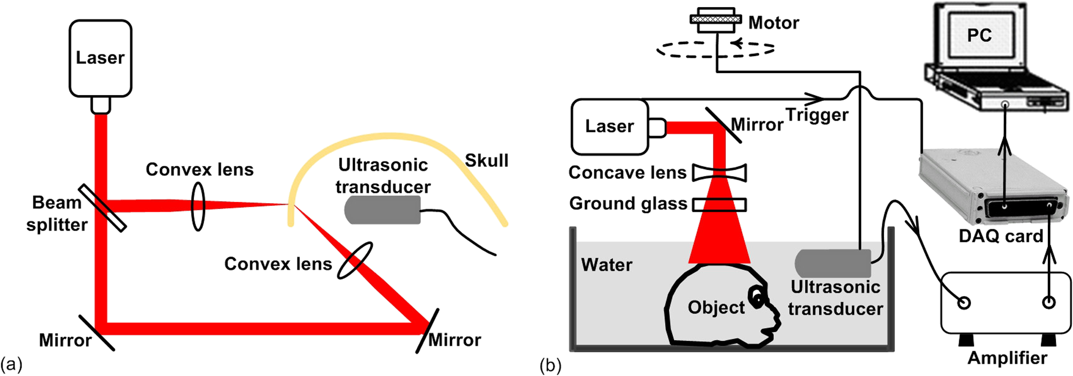
1. Introduction

Photoacoustic tomography (PAT) is a hybrid ultrasound-mediated biophotonic imaging modality that combines the high contrast of optical imaging with the high-spatial resolution of ultrasound imaging.¹^–³ In PAT, biological tissues are illuminated with short laser pulses that results in the generation of internal acoustic wavefields via the thermoacoustic effect. The initial amplitudes of the induced acoustic wavefields are proportional to the spatially variant absorbed optical energy density in the tissue. The acoustic waves propagate through the tissue and are subsequently detected by use of a collection of wide-band ultrasonic transducers that are located outside the object. From knowledge of these data, a reconstruction algorithm is employed to estimate the initial induced pressure distribution or, equivalently if the Grueneisen parameter is known,²^,⁴ the absorbed optical energy distribution within the tissue. Because optical contrast is dependent on hemoglobin concentration and related to the molecular constitution of tissue, PAT can reveal the pathological condition of the tissue,⁵^,⁶ and therefore facilitate a wide-range of diagnostic tasks.⁷^–¹¹

Transcranial brain imaging represents an important application that may benefit significantly by the development of PAT methods. Existing high-resolution human brain imaging modalities such as x-ray computed tomography (CT) and magnetic resonance imaging (MRI) are expensive and employ bulky and generally nonportable imaging equipment. Moreover, x-ray CT employs ionizing radiation and is therefore undesirable for use with patients who require frequent monitoring of brain diseases or injuries. Ultrasonography is an established portable pediatric brain imaging modality, but its image quality degrades severely when employed after the closure of the fontanels. The photoacoustic (PA) signals recorded in a PAT experiment experience only a one-way transmission through the skull. Accordingly, they are generally less attenuated and aberrated than the echo data recorded in transcranial ultrasound imaging, which are contaminated by the effects of a two-way transmission through the skull. Moreover, much of the broadband PA signal energy resides at frequencies less than 1 MHz, and these relatively low-frequencies interact less strongly with skull bone¹² than do higher frequency ultrasound beams that are typically employed in pure ultrasound imaging.

Transcranial PAT studies have revealed structure and hemodynamic responses in small animals¹³^–¹⁵ and anatomical structure in human infant brains have been conducted.¹⁵^–¹⁹ Because the skulls in those studies were relatively thin ( $\sim 1 mm$ ), they did not significantly aberrate the PA signals and conventional back-projection methods were employed for image reconstruction. However, PA signals can be significantly aberrated by thicker skulls present in adolescent and adult primates. To render PAT an effective modality for use with transcranial imaging in large primates, including humans, it is necessary to develop image reconstruction methodologies that can accurately compensate for skull-induced aberrations of the recorded PA signals.

Toward this goal, Xin et al.²⁰ proposed an image reconstruction method that sought to compensate for PA signal aberration associated with acoustic wave reflection and refraction within the skull. In that method, the skull was assumed to be acoustically homogeneous. Accordingly, the method did not explicitly account for scattering effects that arose from heterogeneities in the skull. As a result of the simplified skull model employed, only modest improvements in image quality were observed as compared to use of a standard back-projection-based reconstruction algorithm. Therefore, there remains an important need for the development of improved image reconstruction methodologies for transcranial PAT that are based upon more accurate models of the skull’s heterogeneous acoustic properties.

In this work, we propose and investigate a reconstruction methodology for transcranial PAT that employs detailed subject-specific descriptions of the acoustic properties of the skull to mitigate skull-induced blurring and distortions in the reconstructed image. The reconstruction methodology is comprised of two primary steps. In the first step, the spatially varying speed-of-sound (SOS) and mass density distributions of the to-be-imaged subject’s skull are determined by use of adjunct x-ray CT data. This is accomplished by use of a method that was developed previously to facilitate transcranial adaptive acoustic focusing for minimally invasive brain surgery.²¹ In the second step, the subject-specific SOS and density distributions are employed with a time-reversal image reconstruction method²² for estimation of the spatially variant initial amplitude of the thermoacoustically induced pressure signals within the brain.

The paper is organized as follows. In Sec. 2, the salient imaging physics and image reconstruction principles are briefly reviewed. The image reconstruction methodology is in Sec. 3, which includes a description of how the SOS and density maps of a skull are computed from adjunct x-ray CT data. Section 4 describes the results of the image reconstruction studies that employ a well-characterized phantom and a primate brain, both enclosed in a skull. The paper concludes with a summary and discussion of future work in Sec. 5.

2. Background

Below we briefly review the imaging physics and image reconstruction principles relevant to transcranial PAT imaging. The reader is referred to Refs. 1–3 and 23 for comprehensive reviews of PAT image formation principles.

2.1.

Imaging Physics

The method presented in this work accounts for refraction and diffraction of the photoacoustic wavefields caused by heterogeneities in the SOS and density distributions of the skull. The effects of shear waves propagating in the skull and attenuation of the photoacoustic wavefield in the skull on image formation have not been incorporated in this initial study and represent a topic for future study as discussed in Sec. 5. It should be noted that the density and SOS heterogeneities both have stronger effects and cause more acoustic energy to be reflected back into skull than do the shear wave mode-conversion or attenuation for acoustic plane-wave components incident on the skull surface at small ( $\sim 30 \deg$ or less) angles²⁴ from the surface normal.

Consider tissue that is irradiated by the laser pulse at time $t = 0$ and let $p (r, t)$ denote the induced pressure wavefield at time $t \geq 0$ at location $r$ . When acoustic attenuation and shear wave mode-conversion can be neglected, the following three coupled equations describe the forward propagation of $p (r, t)$ in heterogenous acoustic media:²⁵

Eq. (1)

\frac{\partial}{\partial t} u (r, t) = - \frac{1}{ρ_{0} (r)} \nabla p (r, t),

Eq. (2)

\frac{\partial}{\partial t} ρ (r, t) = - \nabla \cdot ρ_{0} (r) u (r, t),

Eq. (3)

p (r, t) = c_{0} {(r)}^{2} [ρ (r, t) + ξ (r, t) \cdot \nabla ρ_{0} (r)],

subject to the initial conditions:

Eq. (4)

p_{0} (r) \equiv {p (r, t) |}_{t = 0} = Γ (r) A (r), {u (r, t) |}_{t = 0} = 0 .

Here,

A (r)

denotes the absorbed optical energy density within the object,

Γ (r)

is the dimensionless Grueneisen parameter,

u (r, t)

is the acoustic particle velocity,

ξ (r, t)

is the acoustic particle displacement,

c_{0} (r)

denotes the medium’s SOS distribution, and

ρ (r, t)

and

ρ_{0} (r)

describe the distributions of the medium’s acoustic and ambient densities, respectively.

2.2.

Image Reconstruction Based on Time-Reversal

Let ${\hat{p} {(r_{m}, t \in [0, T])}}_{m = 1}^{M}$ denote the measured pressure wavefield data, where $r_{m}$ denotes the location of the $m$ ’th ultrasonic transducer, $M$ indicates the number of measurement locations, and $T$ denotes the maximum time at which the pressure data were recorded. The PAT image reconstruction problem we address is to obtain an estimate of $p_{0} (r)$ or, equivalently, $A (r)$ , from knowledge of ${\hat{p} (r_{m}, t \in [0, T])}_{m = 1}^{M}$ , $c_{0} (r)$ , and $ρ_{0} (r)$ . The development of image reconstruction methods for addressing this problem is an active area of research.²⁶^–²⁸

In this work, we employed a k-space pseudospectral time-reversal image reconstruction algorithm that has been developed by Treeby and Cox.²⁹ The reconstruction algorithm approximates Eqs. (1)–(3), neglecting terms proportional to $\nabla ρ_{0} (r)$ , and solves discretized versions of the three coupled lossless acoustic backward in time with initial and boundary conditions specified as:

Eq. (5)

{p (r, t) |}_{t = T} = 0, {u (r, t) |}_{t = T} = 0, p (r_{m}, t) = \hat{p} (r_{m}, t) .

Unlike the approach proposed by Xin et al.,²⁰ this algorithm is based on a full-wave solution to the acoustic wave equation for heterogeneous media, and can therefore compensate for scattering due to variations in $c_{0} (r)$ and $ρ_{0} (r)$ within the skull. Because the fast Fourier transform (FFT) algorithm is employed to compute the spatial derivatives in the k-space pseudospectral method,²⁹ its computational efficiency is superior to competing methods such as finite-difference time-domain methods. The accuracy of the temporal derivatives can also be refined by use of k-space adjustments.²²

3. Image Reconstruction Studies

Our methodology for aberration correction in transcranial PAT image reconstruction is described below along with details of our experimental studies that involved monkey skulls.

The reconstruction methodology is comprised of two primary steps. First, the spatially varying SOS and density distributions of the to-be-imaged subject’s skull are determined by use of adjunct x-ray CT data. These distributions are subsequently employed with the time-reversal image reconstruction method²² described above for estimation of $p_{0} (r)$ within the brain tissue from knowledge of the measured data ${\hat{p} (r_{m}, t)}_{m = 1}^{M}$ .

3.1.

Description of Biological Phantoms

Two biological phantoms were employed in the experimental studies. The first phantom was the head of an eight-month old rhesus monkey that was obtained from the Wisconsin National Primate Research Center. The hair and scalp were removed from the skull. A second, more simple, phantom was constructed by removing the brain of the monkey and replacing it by a pair of iron needles of diameter 1 mm that were embedded in agar. This was accomplished by cutting off the calvaria to gain access to the brain cavity.

3.2.

Estimation of the Skull’s SOS and Mass Density Distributions from CT Data

The wavefront aberration problem encountered in transcranial PAT is conjugate to one encountered in transcranial focusing of high-intensity ultrasound³⁰^–³² for therapy applications. Both problems involve a one-way propagation of ultrasound energy through the skull and both require that the wavefront aberrations induced by the skull be corrected. The problems differ in the direction of the propagating acoustic wavefields. The feasibility of utilizing skull information derived from adjunct x-ray CT image data to correct for wavefield aberrations in transcranial focusing applications has been demonstrated.²¹ As described below, we adopted this method for determining estimates of $c_{0} (r)$ and $ρ_{0} (r)$ , characterizing the acoustic properties of the subject’s skull, from adjunct x-ray CT data.

3.2.1.

Theory

As described by Aubry et al.,²¹ the SOS and density maps of the skull can be estimated from a porosity map using mixture laws in a biphasic medium (bone/water). Let $H_{k}$ denote the value of the $k$ ’th voxel in the x-ray CT image, which is measured in Hounsfield units. A voxel-based representation of the porosity map, denoted as $ϕ_{k}$ , can be established from knowledge of $H_{k}$ as²¹^,³³

Eq. (6)

ϕ_{k} = 1 - \frac{H_{k}}{H^{Max}},

where

H^{Max}

is the maximum value of

H_{k}

in the CT image.

Let $ρ_{k}$ and $c_{k}$ denote voxel-based representations of the skull’s mass density and SOS distributions. The density map $ρ_{k}$ can be estimated from the porosity map as

Eq. (7)

ρ_{k} = ϕ_{k} ρ^{w} + (1 - ϕ_{k}) ρ^{s},

where

ρ^{w} = 1000 kg / m^{3}

is the density of water, and

ρ^{s} = 2100 kg / m^{3}

is the density of skull as determined by ultrasound experiments.¹²^,²¹ According to Carter and Hayes,³⁴ the elastic modulus of bone is proportional to the apparent density cubed as a first order approximation. This suggests a linear relationship between the speed-of-sound and the porosity:

Eq. (8)

c_{k} = ϕ_{k} c^{w} + (1 - ϕ_{k}) c^{s},

where

c^{w} = 1480 m / s

is the speed-of-sound in water, and

c^{s} = 2900 m / s

is the speed-of-sound of skull bone as determined by previous ultrasound experiments.¹²^,²¹

3.2.2.

Experimental methods

The monkey skull that was part of both phantoms described in Sec. 3.1 was imaged using an x-ray CT scanner (Philips Healthcare, Eindhoven, The Netherlands) located at Washington University in St. Louis. Details regarding this system can be found in Ref. 35. Prior to imaging, three fiducial markers were attached to the skull to facilitate co-registration of the determined SOS and density maps with the reference frame of the PAT imaging system. The three fiducial markers [see Fig. 1(a)] were iron balls of diameter of 1.5 mm and were carefully attached to the outer surface of the skull. The fiducial markers were located in a transverse plane that corresponded to the to-be-imaged 2-D slice in the PAT imaging studies described below. In the x-ray CT studies, the tube voltage was set at 130 kV, and a tube current of 60 μA was employed. Images were reconstructed on a grid of 700 by 700 pixels of dimension $d = 0.1 mm$ . This pixel size is much less than the smallest wavelength (0.5 mm) detected by the ultrasound transducer used in the PAT imaging studies described below. This precision is sufficient to accurately model acoustic wave propagation in the skull by using the k-space pseudospectral methods.³⁶ The reconstructed CT image is displayed in Fig. 1(a).

Fig. 1

(a) A two dimensional slice through the PA imaging plane of the CT of the skull with fiducial markers labeled. (b & c) Speed-of-sound and density maps derived from the CT data using Eqs. (7) and (8) in the PA imaging plane. (d) The PAT image of the monkey head phantom (with brain present) that was reconstructed by use of the half-time algorithm.

From knowledge of the CT image, the porosity map $ϕ_{k}$ was computed according to Eq. (6). Subsequently, the density and SOS maps $ρ_{k}$ and $c_{k}$ were computed according to Eqs. (7) and (8). Images of the estimated $c_{k}$ and $ρ_{k}$ maps are displayed in Fig. 1(b) and 1(c). To corroborate the accuracy of the adopted method for estimating the skull’s SOS and density distributions from x-ray CT data, i.e., Eqs. (7) and (8), direct measurements, of the skull’s average SOS along ray-paths perpendicular to the skull surface at five locations were acquired. This was accomplished by use of a photoacoustic measurement technique depicted in Fig. 2(a). Additionally, the average density of the skull was computed and compared to the average computed from the values estimated from the x-ray CT data. The results show that the directly measured average SOS and density are very close (about 1 to 6%) to the estimated values from CT data. These results corrorborate the adopted method for estimating the skull’s SOS and density distributions from adjunct x-ray CT data. Details regarding these studies are contained in the Appendix.

Fig. 2

(a) A schematic of the transcranial PAT system. (b) A schematic of the PA system for validating the SOS map of the skull.

3.3.

PAT Imaging Studies: Data Acquisition

After the skull’s SOS and density distributions were estimated from the adjunct x-ray CT data, the two phantoms (that included the skulls) were imaged by use of the PAT imaging system shown in Fig. 2(b). Images of the two phantoms with the skull removed, i.e., images of the extracted monkey brain and crossed needles embedded in agar, were also acquired, which will serve as control images. The imaging system employed a 2-D scanning geometry and has been employed in previous studies of PAT imaging of monkey brains.³⁷ The imaging plane and fiducial markers were chosen to be approximately 2 cm below the top of the skull, such that the imaging plane was approximately normal to the skull surface at that plane. The phantoms (crossed needles and the primate cortex) were moved to the imaging plane, so that the amount of acoustic energy refracted out of the imaging plane was minimized. Additionally, the system was aligned to ensure the scanning plane and the imaging plane coincided.

The phantoms were immersed in a water bath and irradiated by use of a tunable dye laser from the top (through the skull for the cases when it was present) to generate PA signals. The laser (NS, Sirah), which was pumped by a Q-switched Nd:YAG laser (PRO-35010, Newport) operating at a wavelength of 630 nm with a pulse repetition rate of 10 Hz, was employed as the energy source. The laser beam was expanded by use of a piece of concave lens and homogenized by a piece of ground glass before illuminating the target. The energy density of the laser beam on the skull was limited to $8 mJ / {cm}^{2}$ (within the ANSI standard), which was further attenuated and homogenized by the skull before the laser beam reached the object.

As shown in Fig. 2, a circular scanning geometry with a radius of 9 cm was employed to record the PA signals. A custom-built, virtual point ultrasonic transducer was employed that had a central frequency of 2.25 MHz and a one-way bandwidth of 70% at $- 6 dB$ . Additional details regarding this transducer have been published elsewhere.³⁷ The position of the transducer was varied on the circular scan trajectory by use of a computer-controlled step motor. The angular step size was 0.9 degrees, resulting in measurement of $\hat{p} (r_{m}, t)$ at $m = 1, \dots, M = 400$ locations on the scanning circle. The total acquisition time was approximately 45 min.

The PA signals received by the transducer were amplified by a 50-dB amplifier (5072 PR, Panametrics, Waltham, MA), then directed to a data-acquisition (DAQ) card (Compuscope 14200; Gage Applied, Lockport, IL). The DAQ card was triggered by the Q-switch signal from the laser to acquire the photoacoustic signals simultaneously. The DAQ card features a high-speed 14-bit analog-to-digital converter with a sampling rate of $50 MS / s$ . The raw data transferred by the DAQ card was then stored in the PC for imaging reconstruction.

3.4.

PAT Imaging Studies: Image Reconstruction

Image reconstruction was accomplished in two steps: (1) registration of the SOS and density maps of the skull to the PAT coordinate system and (2) utilization of a time-reversal method for PAT image reconstruction in the corresponding acoustically heterogeneous medium.

The estimated SOS and density maps $c_{k}$ and $ρ_{k}$ were registered to the frame-of-reference of the PAT imaging as follows. From knowledge of the PAT measurement data, a scout image was reconstructed by use of a half-time reconstruction algorithm.³⁸ This reconstruction algorithm can mitigate certain image artifacts due to acoustic aberrations, but the resulting images will, in general, still contain significant distortions. The PAT image of monkey head phantom (with brain present) reconstructed by use of the half-time algorithm is displayed in Fig. 1(d). Although the image contains distortions, the three fiducial markers are clearly visible. As shown in Fig. 1(a), the fiducial markers were also clearly visible in the x-ray CT image that was employed to estimate the SOS and density maps of the skull. The centers of the fiducial markers in the X-ray CT and PAT images were determined manually. From this information, the angular offset of the x-ray CT image relative to the PAT image was computed. The SOS and density maps were downsampled by a factor of two, to match the pixel size of the PAT images, and rotated by this angle to register them with the PAT images.

The re-orientated SOS and density maps were employed with the k-space time-reversal PAT image reconstruction algorithm developed by Cox et al.²⁸ The numerical implementation of this algorithm provided in the Matlab k-Wave Toolbox²⁹ was employed. The measured PA signals were pre-processed by a curvelet denoising technique prior to application of the image reconstruction algorithm.³⁹ The initial pressure signal, $p_{0} (r)$ , was reconstructed on a grid of $1000 \times 1000 pixels$ of dimension 0.2 mm. For comparison, images were also reconstructed on the same grid by use of a back-projection reconstruction algorithm.⁴⁰ This procedure was repeated to reconstruct images of both phantoms and the corresponding control phantoms (phantoms with skulls removed).

4. Results

4.1.

Images of Needle Phantom

The reconstructed images corresponding to the head phantom containing the needles are displayed in Fig. 3. Figure 3(a) displays the control image of the needles, without the skull present, reconstructed by use of the back-projection algorithm. Figure 3(b) and 3(c) displays reconstructed images of the phantom when the skull was present, corresponding to use of back-projection and time-reversal reconstruction algorithms, respectively. All images have been normalized to their maximum pixel value, and are displayed in the same gray-scale window. Due to the skull-induced attenuation of the high-frequency components of the PA signals, which was not compensated for in the reconstruction process, the spatial resolution of the control image in Fig. 3(a) appears higher than the images in Fig. 3(b) and 3(c). However, the image reconstructed by use of the time-reversal algorithm in Fig. 3(c) contains lower artifact levels and has an appearance closer to the control image than the image reconstructed by use of the back-projection algorithm in Fig. 3(b). This is expected, since the time-reversal algorithm compensates for variations in the SOS and density of the skull while the back-projection algorithm does not.

Fig. 3

(a) The pin-phantom image reconstructed by use of the back-projection algorithm with no skull present. (b & c) The skull-present images reconstructed by use of the back-projection and time-reversal algorithms. (d) Profiles along the white dashed line in each of the three images are shown.

These observations are corrorborated by examination of profiles through the three images shown in Fig. 3(d), which correspond to the rows indicated by the superimposed dashed lines on the images. The solid black, dotted blue, and dashed red lines correspond to the reconstructed control image, and images reconstructed by use of the back-projection and time-reversal algorithms, respectively. The average full-width-at-half-maximum of the two needles in the images reconstructed by use of the time-reversal algorithm is reduced by 8% compared to the corresponding value computed from the images obtained via the back-projection algorithm.

4.2.

Images of Monkey Brain Phantom

The reconstructed images corresponding to the head phantom containing the brain are displayed in Fig. 4. Figure 4(a) displays photographs of the cortex and outer surface of the skull. Figure 4(b) displays the control image (skull absent) reconstructed by use of the back-projection algorithm. The images of the complete phantom (skull present) reconstructed by use of the back-projection and time-reversal algorithms are shown in Fig. 4(c) and 4(d), respectively. All images have been normalized to their maximum pixel value, and are displayed in the same gray-scale window. As observed above for the needle phantom, the brain image reconstructed by use of the time-reversal algorithm in Fig. 4(d) contains lower artifact levels and has an appearance closer to the control image than the image reconstructed by use of the back-projection algorithm in Fig. 4(c).

Fig. 4

(a) Photographs of the brain specimen and skull. (b) The image reconstructed by use of the back-projection algorithm with no skull present. (c & d) The skull-present images reconstructed by use of the back-projection and time-reversal algorithms.

This observation was quantified by computing error maps that represented the pixel-wise squared difference between the control and reconstructed images with the skull present. Figure 5(a) and 5(b) displays the error maps between the control image and the images reconstructed by use of the back-projection and time-reversal algorithms, respectively. The error maps were computed within the region interior to the skull, which is depicted by the red contours superimposed on Fig. 4(b)–4(d). Additionally, the root mean-squared difference (RMSD) was computed by computing the average values of the difference images. The RMSD corresponding to the back-projection and time-reversal results were 0.085 and 0.038. These results confirm that the image reconstructed by use of the time-reversal method, which compensated for the acoustic properties of the skull, was closer to the control image than the image produced by use of the back-projection algorithm.

Fig. 5

Difference images for the brain specimen for reconstructions using back-projection and time-reversal are shown in panels (a) and (b). In both cases, the reference image is the back-projection PAT reconstruction of the brain specimen with the skull removed [see Fig. 4(b)].

5. Summary and Discussion

We have investigated a reconstruction methodology for transcranial PAT that employs detailed subject-specific descriptions of the acoustic properties of the skull to mitigate skull-induced distortions in the reconstructed image. Adjunct x-ray CT image data were employed to infer the spatially variant SOS and density distributions of the skull. Knowledge of these quantities was employed in a time-reversal image reconstruction algorithm to mitigate skull-induced aberrations of the measured PA signals. Our preliminary experimental results, which employed a primate skull, demonstrated that the reconstruction methodology can produce images with improved fidelity and reduced artifact levels as compared to a previously employed back-projection algorithm. This is an important step toward the application of PAT for brain imaging in human subjects.

The use of x-ray CT image data for estimating the skull’s SOS and density distributions was motivated by previous studies of transcranial ultrasound focusing.²¹ Assuming that the skull size and shape does not change, only a single CT scan is required to estimate the SOS and density maps, and does not need to be repeated for subsequent PAT imaging studies of that patient. Because of this, it may be possible to safely monitor brain injuries or conduct other longitudinal studies without repeated exposure to ionizing radiation. Moreover, it may be possible to use adjunct image data produced by alternative modalities such as magnetic resonance imaging⁴¹ or ultrasound tomography⁴² to estimate the required SOS and density maps.

There remain several important topics for future study that may further improve image quality in transcranial PAT. In this preliminary study, to accommodate the 2-D PAT imaging system and 2-D image reconstruction algorithm, the phantoms were moved to the image plane, approximately 2 cm below the top of the skull. Note that this is not the plane in which the cortical vessels are normally found; the primate brain was moved to align the cortical vessels with the imaging plane. For in-vivo transcranial PAT applications in which the cortical structure is of interest, the geometry of the skull necessitates a full 3-D treatment of the image reconstruction problem. The development of robust image reconstruction algorithms for this task is currently underway. Additionally, accurate measurement of the transducer’s electrical impulse response (EIR) and subsequent deconvolution of its effect on the measured data¹¹ would improve image reconstruction accuracy. The possibility also exists that alternatives²⁶^,⁴³ to the time-reversal image reconstruction algorithm employed in this study may yield improvements in image quality.

In terms of the imaging physics, it is expected that development and utilization of image reconstruction algorithms that can compensate for the effects of acoustic attenuation and shear wave mode-conversion will further improve image resolution, particularly for thicker skulls. To date, the manner in which shear waves propagating in the skull affect PAT has only been investigated quantitatively for stratified planar media and planar detection surfaces²⁴^,⁴⁴ via computer-simulation studies. In that case, the effects were observed only in certain high-spatial resolution components of the imaged object. The effects of shear wave propagation and attenuation are both strongly dependent on the thickness of the skull. In this work, the average thickness of the skull was 3 mm and the distortions to the PA signal due to absorption and propagating shear waves were expected²⁴ to be of second-order effect as compared to the distortions due to the variations in the SOS and density. For adult human skulls, where the skull can be $\sim 7 mm$ thick, the relative importance of these effects in transcranial PAT remains to be investigated.

Appendices

Appendix:

Validation of Speed-of-Sound and Density Maps

The density and speed-of-sound of the skull were also directly measured to corrorborate the accuracy of the adopted method for estimating the skull’s SOS and density distributions from x-ray CT data. By using the water displacement method, the measured average density of the monkey skull ${\bar{ρ}}_{w d}$ is $1890 kg / m^{3}$ . The average denisty of the skull ${\bar{ρ}}_{ct}$ can also be estimated from CT data:

Eq. (9)

{\bar{ρ}}_{ct} = \frac{\sum_{k} ϕ_{k} ρ^{w} + (1 - ϕ_{k}) ρ^{s}}{N},

where

ρ^{w} = 1000 kg / m^{3}

is the density of water,

ρ^{s} = 2100 kg / m^{3}

is the density of skull,¹²^,²¹

ϕ_{k}

is the porosity of the

k

’th pixel of the skull, and

N

is the total number of pixels of the skull in the CT image. The estimated average denisty of the skull,

{\bar{ρ}}_{ct} = 1910 kg / m^{3}

is very close (about 1%) to the measured value

{\bar{ρ}}_{w d} = 1890 kg / m^{3}

.

The SOS in the skull was measured using a photoacoustic approach, as shown in Fig. 2(b). A laser beam was split by use of a beam splitter and directed by mirrors to two convex lenses. The two convex lenses ( $NA \approx 0.04$ , depth of focus $\sim 300 mm$ ) focused the laser beam on the inner and outer surface of the skull, and the line connecting the two focused beam spots ( $\sim 80 microns$ ) was perpendicular to the skull surface. The ultrasonic transducer was placed coaxially with the laser spots; therefore, the average SOS ${\bar{c}}_{pa}$ between the two laser spots was calculated by

Eq. (10)

{\bar{c}}_{pa} = \frac{h}{\frac{h}{c^{w}} - t_{d}},

where

t_{d}

is the time delay between the PA signals from the inner and outer surfaces of the skull,

c^{w} = 1480 m / s

is the speed-of-sound in water, and

h

is the thickness of the skull at the laser spots. We measured

{\bar{c}}_{pa}

at the five locations on the skull that are indicated in Fig. 1(a). The measured SOS values are displayed in the second column of Table 1.

Table 1

The measured average SOS c¯pa via the PA experiment (column 2) and the estimated average SOS c¯ct from the CT measurements (column 3) for the five measurement locations [see Fig. 1(a)].

Position	SOS (PA) in m/s	SOS (CT) in m/s
1	$2790 \pm 90$	2720
2	$2740 \pm 80$	2830
3	$2780 \pm 60$	2860
4	$2620 \pm 100$	2720
5	$2590 \pm 160$	2430

The corresponding average SOS values were also computed by use of the x-ray CT image data and compared to the measured values. In order to determine the five locations on the CT image that correspond to the measurement locations described above, we measured the arc lengths between the fiducial markers and the measured locations. Then the average SOS ${\bar{c}}_{ct}$ at these locations can be estimated from CT data [derived from Eq. (8)]:

Eq. (11)

{\bar{c}}_{ct} = \frac{h}{\sum_{i} \frac{d}{ϕ_{i} c^{w} + (1 - ϕ_{i}) c^{s}}},

where

ϕ_{i}

is the porosity of the

i

’th pixels on the line connecting the two laser spots, and is calculated from bilinear interpolation of the neighbor pixel values in the CT image;

c^{s} = 2900 m / s

is the speed-of-sound of skull bone,¹²^,²¹ and

d = 0.1 mm

is the resolution of the CT image. The estimated SOS at these locations are shown in the last column of Table 1. The root mean square difference between the SOS inferred from the PA experiment and the SOS inferred from the CT data is

105 m / s

.

Acknowledgments

Chao Huang, Robert W. Schoonover, and Mark A. Anastasio acknowledge support in part by NIH awards EB010049 and EB009715. Liming Nie, Zijian Guo, and Lihong V. Wang acknowledges support by the NIH awards EB010049, CA134539, EB000712, CA136398, and EB008085. L.V.W. has a financial interest in Microphotoacoustics, Inc. and Endra, Inc., which, however, did not support this work.

References

1.

Photoacoustic Imaging and Spectroscopy, CRC, Boca Raton, Florida (2009). Google Scholar

2.

A. A. Oraevsky, A. A. Karabutov, Biomedical Photonics Handbook, CRC Press LLC, Boca Raton, FL (2003). Google Scholar

3.

M. Xu and L. V Wang, “Biomedical photoacoustics,” Rev. Sci. Instrum., 77 (4), (2006). http://dx.doi.org/10.1063/1.2195024 RSINAK 0034-6748 Google Scholar

4.

V. E. Gusev and A. A. Karabutov, Laser Optoacoustics, AIP, New York (1993). Google Scholar

5.

W. Joines et al., “Microwave power absorption differences between normal and malignant tissue,” Radiat. Oncol. Biol. Phys., 6 681 –687 (1980). http://dx.doi.org/10.1016/0360-3016(80)90223-0 0360-3016 Google Scholar

6.

W. Cheong, S. Prahl and A. Welch, “A review of the optical properties of biological tissues,” IEEE J. Quantum Elect., 26 2166 –2185 (1990). IEJQA7 0018-9197 Google Scholar

7.

M. Xu and L. V. Wang, “Photoacoustic imaging in biomedicine,” Rev. Sci. Instrum., 77 1 –22 (2006). RSINAK 0034-6748 Google Scholar

8.

R. Kruger, D. Reinecke and G. Kruger, “Thermoacoustic computed tomography- technical considerations,” Med. Phys., 26 1832 –1837 (1999). http://dx.doi.org/10.1118/1.598688 MPHYA6 0094-2405 Google Scholar

9.

M. Haltmeier et al., “Thermoacoustic computed tomography with large planar receivers,” Inverse Probl., 20 (5), 1663 –1673 (2004). http://dx.doi.org/10.1088/0266-5611/20/5/021 INPEEY 0266-5611 Google Scholar

10.

B. T. Cox et al., “Two-dimensional quantitative photoacoustic image reconstruction of absorption distributions in scattering media by use of a simple iterative method,” Appl. Opt., 45 (8), 1866 –1875 (2006). http://dx.doi.org/10.1364/AO.45.001866 APOPAI 0003-6935 Google Scholar

11.

K. Wang et al., “An imaging model incorporating ultrasonic transducer properties for three-dimensional optoacoustic tomography,” IEEE Trans. Med. Imag., 30 (2), 203 –214 (2011). http://dx.doi.org/10.1109/TMI.2010.2072514 ITMID4 0278-0062 Google Scholar

12.

F. J. Fry and J. E. Barger, “Acoustical properties of the human skull,” J. Acoust. Soc. Am., 63 (5), 1576 –1590 (1978). http://dx.doi.org/10.1121/1.381852 JASMAN 0001-4966 Google Scholar

13.

G. X. Wang, Y. Pang and L. V. Wang, “Noninvasive laser-induced photoacoustic tomography for structural and functional in vivo imaging of the brain,” Nat. Biotechnol., 21 803 –806 (2003). http://dx.doi.org/10.1038/nbt839 NABIF9 1087-0156 Google Scholar

14.

C. Li et al., “Real-time monitoring of small animal cortical hemodynamics by photoacoustic tomography,” Proc. SPIE, 7564 756427 (2010). http://dx.doi.org/10.1117/12.842159 Google Scholar

15.

Z. Xu, Q. Zhu and L. V. Wang, “In vivo photoacoustic tomography of mouse cerebral edema induced by cold injury,” J. Biomed. Opt., 16 (6), 066020 (2011). http://dx.doi.org/10.1117/1.3584847 JBOPFO 1083-3668 Google Scholar

16.

Y. Xu and L. Wang, “Rhesus monkey brain imaging through intact skull with thermoacoustic tomography,” IEEE Trans. Ultrason. Ferroelectrics Freq. Control, 53 (3), 542 –548 (2006). http://dx.doi.org/10.1109/TUFFC.2006.1610562 ITUCER 0885-3010 Google Scholar

17.

X. Jin, C. Li and L. V. Wang, “Effects of acoustic heterogeneities on transcranial brain imaging with microwave-induced thermoacoustic tomography,” Med. Phys., 35 (7), 3205 (2008). http://dx.doi.org/10.1118/1.2938731 MPHYA6 0094-2405 Google Scholar

18.

X. Yang and L. V. Wang, “Monkey brain cortex imaging by photoacoustic tomography,” J. Biomed. Opt., 13 (4), 044009 (2008). http://dx.doi.org/10.1117/1.2967907 JBOPFO 1083-3668 Google Scholar

19.

L. Nie, Z. Guo and L. Wang, “Photoacoustic tomography of monkey brain using virtual point ultrasonic transducers,” J. Biomed. Opt., 16 (7), 076005 (2011). http://dx.doi.org/10.1117/1.3595842 JBOPFO 1083-3668 Google Scholar

20.

X. Jin, C. Li and L. V. Wang, “Effects of acoustic heterogeneities on transcranial brain imaging with microwave-induced thermoacoustic tomography,” Med. Phys., 35 (7), 3205 –3214 (2008). http://dx.doi.org/10.1118/1.2938731 MPHYA6 0094-2405 Google Scholar

21.

J.-F. Aubry et al., “Experimental demonstration of noninvasive transskull adaptive focusing based on prior computed tomography scans,” J. Acoust. Soc. Am., 113 (1), 84 –93 (2003). http://dx.doi.org/10.1121/1.1529663 JASMAN 0001-4966 Google Scholar

22.

B. E. Treeby, E. Z. Zhang and B. T. Cox, “Photoacoustic tomography in absorbing acoustic media using time reversal,” Inverse Probl., 26 (11), 115003 (2010). http://dx.doi.org/10.1088/0266-5611/26/11/115003 INPEEY 0266-5611 Google Scholar

23.

K. Wang, M. A. Anastasio, Handbook of Mathematical Methods in Imaging, Springer, New York (2011). Google Scholar

24.

R. W. Schoonover, L. V. Wang and M. A. Anastasio, “A numerical investigation of the effects of shear waves in transcranial photoacoustic tomography with a planar geometry,” J. Biomed. Opt., 17 (6), 061215 (2012). http://dx.doi.org/10.1117/1.JBO.17.6.061215 JBOPFO 1083-3668 Google Scholar

25.

P. M. Morse, Theoretical Acoustics, Princeton University Press, Iowa City, IA (1987). Google Scholar

26.

P. Stefanov and G. Uhlmann, “Thermoacoustic tomography with variable sound speed,” Inverse Probl., 25 (7), 075011 (2009). http://dx.doi.org/10.1088/0266-5611/25/7/075011 INPEEY 0266-5611 Google Scholar

27.

Y. Hristova, P. Kuchment and L. Nguyen, “Reconstruction and time reversal in thermoacoustic tomography in acoustically homogeneous and inhomogeneous media,” Inverse Probl., 24 (5), 055006 (2008). http://dx.doi.org/10.1088/0266-5611/24/5/055006 INPEEY 0266-5611 Google Scholar

28.

B. T. Cox et al., “K-space propagation models for acoustically heterogeneous media: application to biomedical photoacoustics,” J. Acoust. Soc. Am., 121 (6), 3453 –3464 (2007). http://dx.doi.org/10.1121/1.2717409 JASMAN 0001-4966 Google Scholar

29.

B. Treeby and B. Cox, “K-wave: MATLAB toolbox for the simulation and reconstruction of photoacoustic wave fields,” J. Biomed. Opt., 15 021314 (2010). http://dx.doi.org/10.1117/1.3360308 JBOPFO 1083-3668 Google Scholar

30.

G. T. Clement and K. Hynynen, “A non-invasive method for focusing ultrasound through the human skull,” Phys. Med. Biol., 47 (8), 1219 (2002). http://dx.doi.org/10.1088/0031-9155/47/8/301 PHMBA7 0031-9155 Google Scholar

31.

J. Sun and K. Hynynen, “Focusing of therapeutic ultrasound through a human skull: a numerical study,” J. Acoust. Soc. Am., 104 (3), 1705 –1715 (1998). http://dx.doi.org/10.1121/1.424383 JASMAN 0001-4966 Google Scholar

32.

J.-L. Thomas and M. Fink, “Ultrasonic beam focusing through tissue inhomogeneities with a time reversal mirror: application to transskull therapy,” IEEE Trans. Ultrason. Ferroelectrics Freq. Contr, 43 (6), 1122 –1129 (1996). http://dx.doi.org/10.1109/58.542055 ITUCER 0885-3010 Google Scholar

33.

M. Pernot et al., “Experimental validation of 3d finite differences simulations of ultrasonic wave propagation through the skull,” in Ultrasonics Symposium, 2001 IEEE, 1547 –1550 (2001). Google Scholar

34.

D. R. Carter and W. C. Hayes, “The compressive behaviour of bone as a two phase porous material,” J. Bone Joint Surg., 59A 954 –962 (1977). 0021-9355 Google Scholar

35.

J. P. Schlomka and E. Roessl et al., “Experimental feasibility of multi-energy photon-counting k-edge imaging in pre-clinical computed tomography,” Phys. Med. Biol., 53 (15), 4031 (2008). http://dx.doi.org/10.1088/0031-9155/53/15/002 PHMBA7 0031-9155 Google Scholar

36.

B. Fornberg, “A practical guide to pseudospectral methods,” A Practical Guide to Pseudospectral Methods, Cambridge University Press, Cambridge, England (1998). Google Scholar

37.

L. Nie, Z. Guo and L. V. Wang, “Photoacoustic tomography of monkey brain using virtual point ultrasonic transducers,” J. Biomed. Opt., 16 (7), 076005 (2011). http://dx.doi.org/10.1117/1.3595842 JBOPFO 1083-3668 Google Scholar

38.

M. A. Anastasio et al., “Half-time image reconstruction in thermoacoustic tomography,” IEEE Trans. Med. Imag., 24 199 –210 (2005). http://dx.doi.org/10.1109/TMI.2004.839682 ITMID4 0278-0062 Google Scholar

39.

E. Candes, “The curvelet transform for image denoising,” in Image Processing, 2001. Proc. 2001 International Conf. on, 7 (2001). Google Scholar

40.

C. Li, G. Ku and L. V. Wang, “Negative lens concept for photoacoustic tomography,” Phys. Rev. E (Statistical Physics, Plasmas, Fluids, and Related Interdisciplinary Topics), 78 021901 (2008). http://dx.doi.org/10.1103/PhysRevE.78.021901 PLEEE8 1063-651X Google Scholar

41.

J. Hong et al., “Magnetic resonance imaging measurements of bone density and cross-sectional geometry,” Calcif. Tissue Int., 66 74 –78 (2000). http://dx.doi.org/10.1007/s002230050015 CTINDZ 0171-967X Google Scholar

42.

J. Ylitalo, J. Koivukangas and J. Oksman, “Ultrasonic reflection mode computed tomography through a skullbone,” IEEE Trans. Biomed. Eng., 37 (11), 1059 –1066 (1990). http://dx.doi.org/10.1109/10.61031 IEBEAX 0018-9294 Google Scholar

43.

P. Stefanov and G. Uhlmann, “Thermoacoustic tomography arising in brain imaging,” Inverse Probl., 27 045004 (2011). http://dx.doi.org/10.1088/0266-5611/27/4/045004 INPEEY 0266-5611 Google Scholar

44.

R. W. Schoonover and M. A. Anastasio, “Compensation of shear waves in photoacoustic tomography with layered acoustic media,” J. Opt. Soc. Am. A, 28 (10), 2091 –2099 (2011). http://dx.doi.org/10.1364/JOSAA.28.002091 1084-7529 Google Scholar

Citation Download Citation

Chao Huang, Liming Nie, Robert W. Schoonover, Zijian Guo, Carsten O. Schirra, Mark A. Anastasio, and Lihong V. Wang "Aberration correction for transcranial photoacoustic tomography of primates employing adjunct image data," Journal of Biomedical Optics 17(6), 066016 (5 June 2012). https://doi.org/10.1117/1.JBO.17.6.066016

Received: 14 January 2012; Accepted: 12 April 2012; Published: 5 June 2012

Access the abstract

JOURNAL ARTICLE
8 PAGES

DOWNLOAD PAPER SAVE TO MY LIBRARY

GET CITATION

CITATIONS

Cited by 86 scholarly publications and 9 patents.

Explore citations on Lens.org

RIGHTS & PERMISSIONS

Get copyright permission Get copyright permission on Copyright Marketplace

KEYWORDS

Skull

Reconstruction algorithms

Acquisition tracking and pointing

Image restoration

Acoustics

X-ray computed tomography

X-rays

1.

Introduction

2.

Background

2.1.

Imaging Physics

Eq. (1)

Eq. (2)

Eq. (3)

Eq. (4)

2.2.

Image Reconstruction Based on Time-Reversal

Eq. (5)

3.

Image Reconstruction Studies

3.1.

Description of Biological Phantoms

3.2.

Estimation of the Skull’s SOS and Mass Density Distributions from CT Data

3.2.1.

Theory

Eq. (6)

Eq. (7)

Eq. (8)

3.2.2.

Experimental methods

Fig. 1

Fig. 2

3.3.

PAT Imaging Studies: Data Acquisition

3.4.

PAT Imaging Studies: Image Reconstruction

4.

Results

4.1.

Images of Needle Phantom

Fig. 3

4.2.

Images of Monkey Brain Phantom

Fig. 4

Fig. 5

5.

Summary and Discussion

Appendices

Appendix:

Validation of Speed-of-Sound and Density Maps

Eq. (9)

Eq. (10)

Table 1

Eq. (11)

Acknowledgments

References

Show All Keywords

Keywords/Phrases

Search In:

Publication Years