2.1.

Sample Preparations

Red-orange carboxylate-modified 40-nm-diameter fluorescent spheres having excitation/emission maxima at $565/580\mathrm{nm}$ were from Molecular Probes (Life Technologies, Grand Island, NY). The stock was diluted ${10}^4$-fold into distilled water, giving a concentration of $1.4\times {10}^{11}\text{spheres}/\mathrm{mL}$. Experiments were conducted at room temperature.

Experiments were performed in microfluidic channels constructed using the toner transfer method just as described earlier.¹¹ Figure 1(a) shows the channel pattern drawn in Adobe Photoshop at 1200-dpi resolution with each square pixel $\sim 20\mu \text{\hspace{0.17em}m}$ on a side. Horizontal stripes are 100 µm wide, and the full pattern fits on a 22- by 30-mm #1 glass coverslip ($\sim 0.15\mathrm{mm}$ thick). The pattern was printed onto Toner Transfer Paper (Pulsar, Crawford, FL) using a Samsung Laserjet printer (model ML-3471ND) at 1200-dpi printing resolution. The pattern was transferred to a brass substrate cut from shim stock (0.032 inch thick, Amazon) using heat and brass etching performed with a 20% solution ($\mathrm{w}/\mathrm{v}$) of ammonium persulfate (APS, Sigma). Regions protected by the toner are not etched. The pattern was etched to a depth of 20 µm using the total substrate weight to monitor progress, and the depth was verified experimentally as described below.

Fig. 1

Master pattern and assembly of the microfluidic chamber. (a) The master pattern drawn in Adobe Photoshop and printed onto toner transfer paper. Lines are 100 µm wide and 30 mm long. The pattern is transferred to a brass blank that is etched in APS. (b) Component assembly for making the PDMS spacer. Brass master has 20 µm deep channels filled with unpolymerized PDMS. After assembly, the multilayered system is clamped between 0.25-inch thick aluminum stock plates (Al) then heated to polymerize the PDMS. The spacer remains firmly attached to the coverslip but detaches from the brass master. (c) The completed microfluidic chamber formed from the coverslip, polymerized PDMS, and another coverslip placed on the top. Fluorescent spheres were dried down on the top coverslip before it was put on top of the chamber. Water was also added to fill the chamber before the top was put into place. Some spheres from the top coverslip detach and settle onto the bottom coverslip.

Polydimethylsiloxane (PDMS) was poured over the brass master, then a #1 glass coverslip was placed on top with care taken to avoid trapping air bubbles under the coverslip. A glass slide covered the coverslip but with immersion oil in between to prevent the coverslip sticking to the slide. Next a cardboard pad evenly distributed pressure from the 0.25-inch-thick aluminum stock plates (Al) as shown in Fig. 1(b). The assembly was clamped with a 1-inch binder clip, then heated to 80°C for 2 h to polymerize the PDMS as described previously.¹² After heating, the assembly was broken down and the coverslip recovered. On separating the coverslip from the brass master, the 20-µm-thick PDMS pattern tightly and smoothly adhered to the glass.

A watertight chamber was constructed from 3 coverslips. Two coverslips formed the top and bottom of the chamber, and the third was used to make 2- by 30-mm spacers separating the top and bottom coverslips. The spacers were arranged along the long edges of the coverslips. The spacers and coverslips formed a 0.15-mm-thick rectangular solid volume with opposite ends open. Fluorescent spheres were flowed into the open ends of the sample chamber and allowed to dry. A drop of distilled water was placed on the PDMS pattern—covered coverslip, then the bottom coverslip with dried fluorescent spheres attached was placed on top, sphere side down. The PDMS pattern and glass coverslip sandwich [see Fig. 1(c)] was placed on a slide holder with the PDMS-fixed coverslip on the bottom. The slide holder had a large hole cut out to allow access by the objective from the inverted microscope. After $\sim 30\min$, a sparse random distribution of fluorescent spheres was observed in the microscope, fixed to either the upper or lower glass surface. The surfaces were 20 µm apart, judging by the distance the objective traveled to move focus between the lower and upper surfaces. Spheres diffusing in solution were rarely observed with the objective focused on either glass surface. Most experiments were performed on fluorescent spheres fixed to the lower coverslip in optical contact with the objective. Some experiments were performed on fluorescent spheres fixed to the upper coverslip. The latter were separated from the lower coverslip by the 20-µm aqueous layer and were well beyond the evanescent field present at the lower coverslip. Fluorescent spheres were always in the aqueous medium.

2.2.

Microscopy

Figure 2 shows the inverted microscope (Olympus IX71) with excitation and emission detection pathways. Double arrows indicate translating elements in the apparatus with their approximate spatial resolution. The 514.5-nm line from the argon ion laser (Innova 300, Coherent, Santa Clara, CA) is intensity modulated by the acoustoptic modulator (AOM) then linearly polarized by the Glan-Taylor (P) polarizer. The polarization rotator (PR) uses Fresnel Rhombs to rotate linearly polarized light to the desired orientation. Linearly polarized light, split into two beams at the interferometer (IF), travels different path lengths before rejoining. Path length difference is $\sim 4\mathrm{cm}$, well under the $\sim 10\mathrm{cm}$ coherence length of the laser. The lower and upper path beams have relative path difference controlled to $\sim 1\text{-}\mathrm{nm}$ precision using a nanopositioning piezo stage and controller (nano-bio 100, MCL, Madison, WI) that translates two mirrors in tandem within the box. The beam expander (BE) consists of a $4\times$ or $10\times$ microscope objective and a large-diameter, long-focal-length (250 mm) lens (LFL). The LFL translates with 25-μm resolution using a motorized micrometer (Newport, Irvine CA). Exciting laser light enters the microscope, reflects at the dichroic mirror (DM), and is focused on the sample by the objective. The objective (Olympus planapo $60\times$, 1.45 NA, and 100 µm working distance) translates along the optical axis under manual control using the microscope focus and with nanometer precision using a piezo nanopositioner (C-Focus, MCL). Emitted light is collected by the objective, transmitted by the dichroic mirror, then focused by the tube lens (TL) onto the camera (CCD, Orca ER, Hamamatsu Photonics, Hamamatsu-City, Japan). A microscope stage with leadscrew drives and stepper motors translates the CCD camera with submicrometer resolution (LEP, Hawthorne, NY).

Fig. 2

Optical train for excitation and emission detection pathways serving the Olympus IX71 microscope. Double arrows indicate translating elements with the approximate spatial resolution indicated. Abbreviations: acoustoptic modulator (AOM), mirror (M), Glan-Taylor polarizer (P), polarization rotator (PR), interferometer (IF), beam expander (BE) containing the long focal length lens (LFL), dichroic mirror (DM), tube lens (TL), and CCD camera.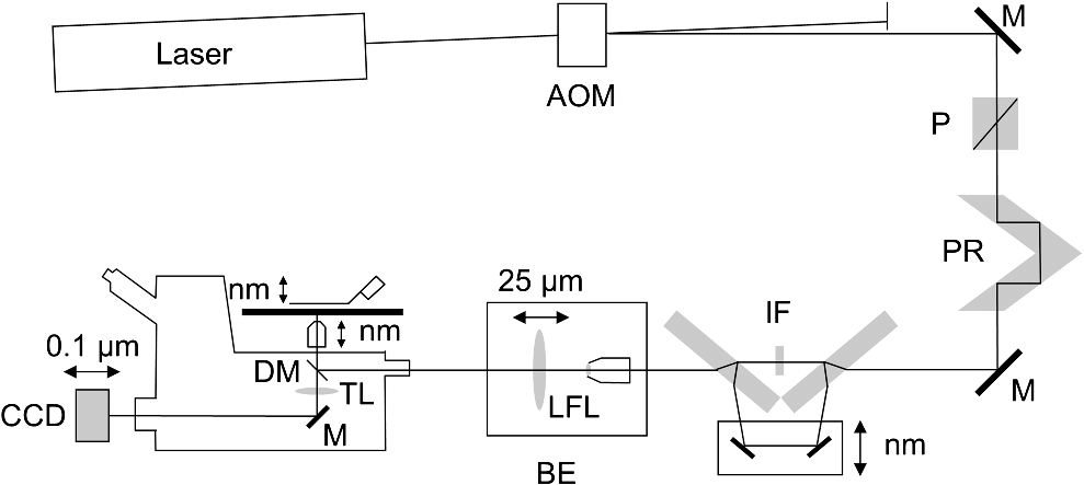

Overall computer control of the microscope is exercised through a custom-written Labview (National Instruments, Austin TX) routine and drivers supplied by the manufacturers. The Labview software coordinates image capture by the camera with movement of the various translating elements in or around the microscope. Translating elements are controlled via a RS232 port (LEP stage), a USB interface (MCL nanopositioners), or a D/A channel (NI6024 controlling the motorized micrometer driver). HCImage (Hamamatsu) captures the images following triggering by the main Labview program via a counter output TTL pulse (NI6602).

An oil-immersion objective with a coverslip separating objective and aqueous sample and with NA larger than the refractive index of water ($\sim 1.3$) will produce superpositioned evanescent and propagating fields on the aqueous side under epi-illumination when axial rays fill the BFP. Through-the-objective total internal reflection fluorescence (TIRF) confines the illuminating beam to regions in the BFP where only evanescent illumination will be produced at the sample.¹³

2.3.

Interferometer

Figure 3 details the interferometer. Incident light propagates along the $z$-axis with incident and reflected beams confined to the $\mathrm{xz}$-plane. Transparent gray slabs are glass optical flats of thickness $L_1$. Light incident at angle $\sigma$ transmits the air/glass interface then transmits (primary arm) or reflects (reflected arm) at the glass—air interface with the unbroken line depicting light paths. Broken lines indicate some of the uncaptured alternative light pathways. Neutral-density filter (NDF) slightly lowers intensity to balance primary and reflected beam intensities. Linear polarization is s-polarized at the flats in all experiments. Distance $L_2$ is the closest distance from mirror $M$ and the optical flat. Air has refractive index $n_1$ and glass $n_2$. Distances $d_i$ define the path lengths traveled by the primary and reflected beams.

Fig. 3

The interferometer. Opposing glass optical flats of thickness $L_1$ split the laser beam into transmitted (primary) and reflected beams that follow different paths then rejoin before propagating to the beam expander. Solid lines indicate the paths of primary and reflected beams. The neutral density filter (NDF) has 0.05 absorbance to approximately balance the final intensities of the two beams. Other parameters relevant to the path length difference calculation for primary and reflected beams are listed [see Eqs. (1) and (2) in the text]. Mirrors (M) are translated along $x$ with nanometer resolution to affect path length in the reflected beam.

Path-length difference between primary and reflected beams, $\mathrm{\Delta }$, is given by

2.4.

Computation of Field Intensity Propagating through a Lens

Exciting and emitted fields are computed using an integral representation of the fields transmitting a lens.¹⁴ The exciting light propagates parallel to the optical axis and refracts at the objective, producing a focused spot. Emitted light originates from near the microscope objective focal plane and emerges after refraction as plane polarized rays propagating toward the tube lens. The tube lens reverses the process and forms the magnified image on the CCD camera. Lateral magnification determines the size of the image in the camera detector plane. Axial magnification is the distance the camera must translate axially to refocus an object translated from the objective focal plane. Microscope optics obeying Abbe’s sine condition are assumed such that finite conjugate excitation illumination, or axial displacement of the fluorescent object from focus, introduces spherical aberration to the image.

2.5.

Computation of Excitation Field Intensity

A Gaussian laser beam impinges on the objective via the epi-illumination port with the ratio of objective aperture radius, $a_0$, to beam waist radius, $w_0$, given by $\beta =a_0/w_0$.¹⁵ A light ray from the Gaussian beam propagates in object space parallel to and at a distance $h$ from the optical axis toward the objective aperture. The refracted ray propagates in image space in the direction of the unit vector $\widehat{s}$ making an angle $\theta$ with the optical axis. The meridional plane is formed by the ray in object and image space. The angle between the meridional plane and the incident electric field is conserved following refraction by the objective. After refraction at the objective, the ray transmits the coverslip of the oil-immersion objective with efficiency given by the Fresnel coefficients. In the two-beam configuration, electric fields from primary and reflected beams are computed then superimposed.

The axial path difference between the primary and reflected beams produces a relative phase shift that manifests as an interference pattern near the focus as the phase shift nears odd multiples of half the exciting light wavelength. Some calculations were performed for crossed primary and reflected beams with a lateral phase difference that produces an interference pattern in the lab-fixed $\mathrm{xy}$-plane ($\mathrm{xz}$-plane indicated in Fig. 3). A diffraction pattern due to interference between two crossed Gaussian beams gives a field amplitude proportional to $\cos (\frac{\pi }{2}\frac{x}{\mathrm{\Delta }})$ where $x=h\cos \varphi$, $\varphi$ is the azimuthal angle of the meridional plane, and $\mathrm{\Delta }$ is the distance in the $x$-dimension separating zero-intensity nodes (measured after the beam expander). Path-length difference between the crossed beams indicates

Crossed beams in the $\mathrm{xz}$-plane produce a lateral interference pattern with zero-intensity nodes in columns projecting into the lab frame $y$-dimension (Fig. 3). The $\mathrm{xy}$-plane pattern was observed on a white card placed after the beam expander to confirm laser beam coherence. Adjusting the two-beam propagation directions to near collinearity spreads the pattern out beyond the laterally illuminated region. Equation (3) indicates $\gamma$ 0.075 deg. The small crossing angle does not substantially affect computed intensity profiles shown subsequently. The minimal $\gamma$ 0.075 configuration was used for all measurements.

2.6.

Finite Conjugate Illumination

The beam expander shown in Fig. 2 (BE) expands the excitation beam waist using a low-power ($4\times$ or $10\times$) microscope objective and the LFL with focal lengths of 2 or 25 cm, respectively. Translation of the LFL provides infinite or finite conjugate illumination of the objective. Infinite conjugate illumination is a collimated beam focused by the objective at its focal point (although for two-beam incidence the intensity at focus can be at a minimum). Finite conjugate illumination involves a slightly convergent or divergent beam that axially shifts the real image. For two-beam incidence, finite conjugate illumination could axially shift the intensity peaks offset from the focus such that one of them can be coincident with the objective focus at the origin. Shifted intensity peaks are useful for sample illumination but suffer from spherical aberration as described.⁵ There it is shown that finite conjugate illumination has aberration $W$, given by

2.7.

Computation of Emission-Field Intensity and Detected Image

Divergent light collected by the objective converts to plane-polarized light rays propagating in parallel in image space toward the tube lens. Intensity patterns at the BFP represent the angular divergence of collected rays as a spatial intensity pattern separating the near-field from far-field emission of the fluorescent object.⁸ The BFP spatial intensity pattern from single-molecule fluorescence emission also uniquely quantifies emitter dipole orientation.⁹ The image space propagating light transmits the dichroic and barrier filters that impact the light polarization and the intensity pattern ultimately imaged by the tube lens on the CCD. The tube lens was air immersion with 180-mm focal length and radius of 12.5 mm in the IX71. The computation of the emitted field as it transmitted the objective, dichroic filter, tube lens, and then imaged on the camera was described previously.¹⁰

The emitted field at the CCD camera is the superposition of contributions from the emission dipole components. Like the lateral dependence, emitted field intensity axial dependence distinguishes emission from dipoles that are in the object plane (parallel) or normal to it (normal). Figure 4 indicates the emitted field intensity axial dependence from a normal (solid line) or parallel (dashed line) dipole. Normal dipole emission intensity approaches zero (compared to a parallel dipole) precisely at its image space focal point; however, the camera pixel integrates over a finite area in the image plane. Figure 4 shows an integrated intensity over the domain of a single CCD camera pixel. In this case, intensities are comparable between normal and parallel dipoles. Figure 4 also indicates that peak intensities differ for parallel and normal components. It is an aberration that is minimized but not eliminated by the objective compensating collar.

Fig. 4

Axial emission intensity profile at the CCD camera. Emitted fields from a single chromophore are the superposition of contributions from the emission dipole components. Emission dipoles in the object plane (parallel) or normal to it (normal) have different profiles given by the dashed or solid black lines. The generic profile (dot-dashed) is the standard model that does not distinguish between dipole components. Axial position of peak intensities differs for parallel and normal components.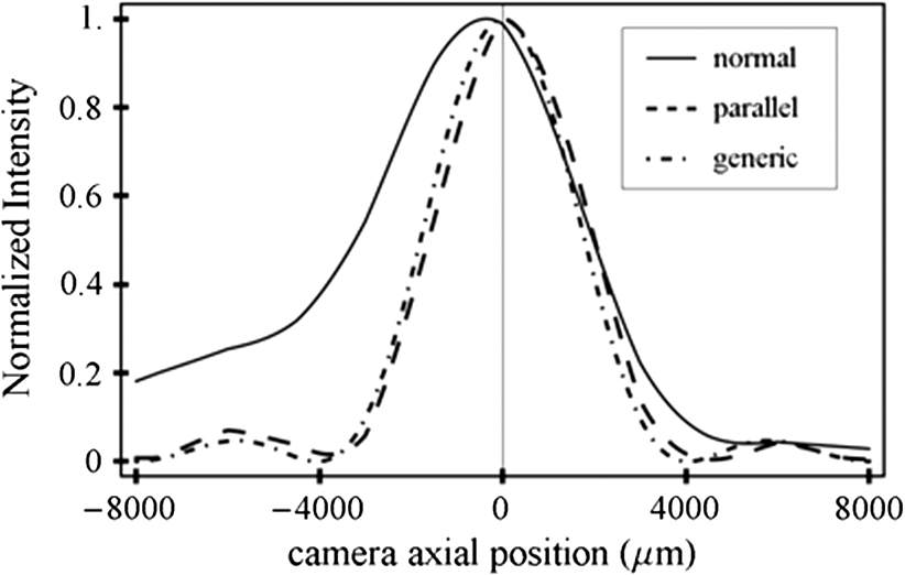

Alternatively, the axial emitted intensity is nominally approximated by a dipole orientation—independent profile¹⁶ given by

The axial profile from Eq. (6) is labeled “generic” in Fig. 4.

3.1.

Excitation Intensity Profile Versus Proximity to the Interface

Comparing axial epi-illumination excitation profiles for points inside the aqueous medium shows the evanescent field effect on intensity. Calculation shows that when $\beta =0.8$ and for an exciting wavelength of 514.5 nm, an object on the coverslip interface sees an intensity profile with characteristic FWeM lengths of {380, 230, 368} nm for $x$-, $y$-, and $z$-dimensions. Linearly polarized incident electric field on the $x$-axis correlates with the widest profile. The $y$-dimension profile is significantly shorter than the others by close to a factor of 2. The axial dimension is intermediate but practically equal to the $x$-dimension profile. This contrasts with FWeM lengths of {382, 256, 518} nm seen by an object 20 µm from the coverslip interface in the aqueous medium but under otherwise identical conditions. In calculations, the evanescent field has a small effect on the lateral dimensions and a strong effect on the axial dimension. Axial FWeM length vs distance from the interface is plotted in Fig. 5. For objects on the interface, the axial half width at $1/e$ times maximum is 184 nm, which compares to the $\sim 100\text{-}\mathrm{nm}$ depth of the evanescent field intensity in TIRF microscopy.¹⁷

Fig. 5

Exciting light intensity axial half width at $1/e$ times maximum height versus distance from the interface for a point object detected with the 1.45-NA TIRF objective. The value at zero distance is for an object on the coverslip where the evanescent field is maximal.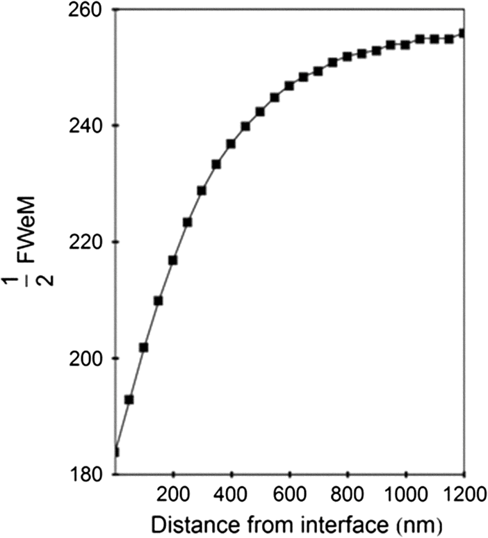

I measured intensity profiles using the IX71 microscope, the $60\times$, 1.45-NA objective, and 40-nm-diameter fluorescent spheres immobilized on a glass surface, as described in Sec. 2. Experiments were conducted by focusing the objective on a fluorescent sphere specimen then translating the objective axially through a sawtooth pattern using the C-focus nanopositioner. Translation sweeps the exciting intensity profile through the point source that fluoresces proportionally to the exciting intensity. Figure 6 shows the objective translation sawtooth pattern (solid line) and the intensity observed for a one-beam (primary only) exciting light configuration (solid square). The righthand abscissa scale applies to the sawtooth curve with tickmarks indicating objective axial position. The lefthand abscissa scale applies to the intensity. In subsequent figures plotting the objective axial position (independent variable) versus fluorescence intensity (dependent variable), only the middle portion of the sawtooth pattern is shown where objective position changes monotonically. The translating objective emission profile used for simulating curves is the generic axial profile in Eq. (6) while neglecting aberration. The emission axial profile for the 1.45-NA objective is substantially broader than distinctive features in the excitation profiles and negligibly impacts fitting.

Fig. 6

Objective translation sawtooth pattern (solid line) and the intensity observed for a one-beam (primary only) exciting light configuration (solid square). The righthand abscissa scale applies to the sawtooth curve indicating objective position. The lefthand abscissa scale applies to the collected intensity in arbitrary units.

Both one- and two-beam configurations were used. Primary and reflected beams in the two-beam configurations had approximately equal intensities. The two-beam configurations, compared to their one-beam counterparts, provided more features to be aligned with simulation to enhance fitting reliability. Fitted curves (solid lines) for the two-beam configurations were generated as described in Sec. 2 with $\delta$ (relative phase shift between primary and reflected beams) and relative intensities of primary and reflected beams used as free parameters. In the one-beam configuration, there are no free fitting parameters. However, for either configuration, $\beta$ is allowed to vary within $\sim 20\%$ of its nominal value of 0.8 or 2 for the $10\times$ or $4\times$ objective in the beam expander.

Figure 7 shows measured and simulated intensity profiles for the one-beam configuration and compares profiles from objects fixed to the lower or upper glass coverslip (see Fig. 1). Point fluorescent objects on the lower coverslip, where both evanescent and far fields contribute to excitation, produce the narrower profile (solid square). Point fluorescent objects on the upper coverslip produce the broader profile (open square). They are 20 µm from the lower coverslip across an intervening water layer and are subjected only to the far field. Computed profiles (solid lines) use $\beta =2$ and differ only because of the evanescent field at the lower coverslip. Relative intensity between fluorescent point sources fixed to the lower and upper coverslips, not documented by the normalized intensity curves, is 2- to 4-fold higher at the lower coverslip where the evanescent field is present. Unpredicted oscillation of intensity near the extreme upstream objective translation may be due to aberration.

Fig. 7

Measured and simulated (solid line) exciting intensity profiles for the one-beam configuration and comparing profiles from fluorescent objects fixed to the lower (solid square) or upper (open square) glass coverslip. The narrower profile is in the presence of the evanescent field.

Figure 8 shows measured and simulated intensity profiles in several exciting light configurations all at the lower coverslip. Figure 8(a) shows intensity profiles for $\beta =2$ and one-beam (primary only, open square) or two-beam (primary and reflected interfering, solid square) configurations. The computed one-beam profile has 1291 nm FWeM. According to simulation, the curve from the two-beam configuration corresponds to $\delta =7\lambda /2$. The profile peaks broaden and separate with increasing $\delta$. Relative beam intensity in the simulation for the two-beam configuration was 0.45 (primary) and 0.55 (reflected).

Fig. 8

Measured and simulated exciting intensity profiles in several exciting light configurations all for a fluorescent object at the lower coverslip. (a), Intensity profiles for $\beta =2$ and one-beam (open square) or two-beam (solid square) configurations. The two-beam configuration corresponds to relative phase shift $\delta =7\lambda /2$. (b), The intensity profile for $\beta =2$ and two-beam configuration with $\delta =\lambda /2$. (c), The intensity profile for $\beta =0.8$ and two-beam configuration with $\delta =\lambda /2$. This is the narrowest observed profile, with $\sim 250\mathrm{nm}$ peak separation. Simulation does not accommodate key profile features including the main peak resonance positions and widths and the side resonance beyond the main peaks at 500 nm.

Figure 8(b) shows the intensity profile for $\beta =2$ and two-beam configuration with $\delta =\lambda /2$. The profile has narrow peaks and $\sim 450\text{-}\mathrm{nm}$ peak separation in agreement with simulation. A primary-only configuration has a 1006-nm FWeM axial profile in simulation (not shown). The dominant features of the observed profile are reproduced in simulation. Relative beam intensity in the simulation for the two-beam configuration was 0.47 and 0.53.

Figure 8(c) shows the intensity profile for $\beta =0.8$ and two-beam configuration with $\delta =\lambda /2$. This is the narrowest observed profile, with $\sim 250\mathrm{nm}$ peak separation. Simulation is unable to match the key profile features, including the main peak resonance positions and widths and, in particular, the side resonance that appears at $\sim 500\mathrm{nm}$. A primary-only configuration has a 368-nm FWeM axial profile in simulation (not shown). Relative beam intensity in the simulation for the two-beam configuration was 0.5 and 0.5.

Simulation width in the axial dimension is strongly influenced by the evanescent field at the interface such that the profile narrows as the evanescent field contribution increases (Fig. 5). Results in Fig. 8(c) suggest that simulation underestimates the evanescent field effect, possibly because the planar model for the coverslip/aqueous interface is inadequate for the narrowest profile where the evanescent field effect is expected to be largest. Axial epi-illumination at the BFP falls within and without the critical angle ring dividing far- and evanescent-field exciting light, respectively, after refraction in the objective. The $\beta =0.8$ BFP illumination has more of the total illumination falling beyond the critical angle ring, hence producing more evanescent exciting light. The 40-nm-diameter fluorescent sphere on the interface could enhance or focus evanescent field intensity in its vicinity that is more readily detected in the $\beta =0.8$ profile.

3.2.

Adapting the Exciting Intensity Profile

Figure 9 shows the measured exciting light intensity profile swept through the objective focus by using finite conjugate illumination and the fitted profile computed using Eqs. (4) and (5) and $\beta =2$. Experiments were conducted by focusing the objective on a fluorescent sphere specimen at the lower coverslip using the primary-only exciting beam configuration then returning to the two-beam configuration and sweeping the LFL through a sawtooth pattern like that in Fig. 6. Shown is the emission intensity from the fluorescent sphere in the central section of the sawtooth where the LFL moves away from the microscope monotonically. The exciting light intensity profile is strictly proportional to fluorescence detected, confirming the bimodal axial intensity distribution for the two-beam configuration. The objective is not translating axially, hence no emission profile or emission aberration is involved; however, there is aberration in the exciting profile as discussed previously⁵ that I fully account for in simulation. The LFL translates the exciting light axial profile such that the peak intensity and emission focal plane are brought into coincidence. Figure 9 demonstrates the good agreement between computed and observed intensity profiles, indicating accurate modeling of the optical system. The profiles also show that the excitation and emission focal planes can be adjusted independently using the LFL and the objective correction collar in concert.

Fig. 9

Measured (solid square) and simulated (solid line) exciting light intensity profile vs position of long focal length lens (LFL) in the beam expander (Fig. 2). The LFL adapts the two-beam configuration excitation such that the exciting light peak intensity and emission focal plane are brought into coincidence at the fluorescence peaks. The LFL translates monotonically away from the microscope in its 25-mm travel.

3.3.

Image Space Emission Profile

Figure 10 shows the detected axial dependence of the image field at the lateral focal point pixel from a 40-nm-diameter sphere fixed on the lower coverslip/aqueous interface (solid square). Experiments were conducted by CCD camera translation as described in Sec. 2, where light impinging on the center pixel of the sphere image is followed as the camera is scanned axially over $\sim 10\mathrm{mm}$ using the LEP stage. Solid line curves are best fits estimated using Eq. (6) (dashed line) or by the integral representation (solid line) of the image field. The latter best accounts for observation and provides best-fit parameters for a linear combination of the emitting dipole components normal (78%) or parallel (22%) to the coverslip/aqueous interface.

Fig. 10

Measured (solid square) and simulated (solid or dashed lines) axial dependence of the image field at the lateral focal point pixel from a 40-nm-diameter sphere fixed on the lower coverslip/aqueous interface. Light impinging on the center pixel of the sphere image is plotted as the CCD camera is scanned axially over $\sim 10\mathrm{mm}$. Best-fitting curves were generated for the integral representation (solid line) of the image field and from Eq. (6) (dashed line). The integral representation best accounts for observation.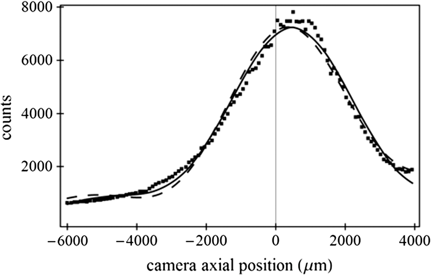

The exciting evanescent field supports a large normal polarization component that varies from near zero to 70% of total intensity within $\sim 1/e$ of the peak intensity. A small sphere at the lower coverslip can experience almost twice the normally polarized light (depending on exact lateral position) as the same sphere at the upper coverslip owing to the dominance of the evanescent field. For a random distribution of probes, which I assume is the case for a fluorescent sphere conjugated to many chromophores, the observed fluorescence intensity follows the breakdown of exciting light polarization intensity. My image space emission profile analysis, summarized in Fig. 10, supports the higher normal component present in the total exciting field due to the evanescent field at the lower coverslip.