Neurological disorders are prevalent worldwide and have been seriously underestimated by established epidemiological analysis methods.¹ The World Health Organization has drawn the attention of the international health community to the fact that, even though neurological disorders are responsible for approximately 1% of deaths, they account for almost 11% of health burdens worldwide. Therefore, developing new high-performance optical imaging technology is a key to better understanding of the underlying mechanisms of brain diseases. The significant advances in optical coherence imaging offer broad potential for imaging from cellular to tissue levels, with promising applications in humans.

Recently, several research groups have demonstrated optical coherence tomography (OCT) methods to visualize major cortical vessels in adult rodents. Wang et al. used optical micro-angiography to visualize three-dimensional (3-D) cerebral circulation in living adult mice.² An optical frequency domain imaging technique was introduced by Vakoc et al. to measure angiogenesis rapidly and repeatedly in mouse tumors.³ Finally, Srinivasan et al. used Doppler OCT (DOCT) and angiography to image the rat cerebral cortex.⁴ Most of these techniques focus on the visualization of cerebral vasculature by using intrinsic scattering contrast alone. However, the measurement of cerebral blood flow is an important endpoint in the study of cerebral pathophysiology. Wang et al.² and Srinivasan et al.⁴ have demonstrated algorithms to receive complementary information about blood flow in rodent vessels. The main challenge is a wide range of flow velocities that can range from tens of $\mathrm{mm}/\mathrm{s}$ in large blood vessels to fractions of $\mathrm{mm}/\mathrm{s}$ in capillary networks. Assessment of such a wide velocity range is difficult to achieve using DOCT. Imaging methods and scanning protocols must be developed to obtain quantitative information about blood flow velocity and high-sensitivity maps of capillary networks.⁵

We would like to propose a method of qualitative and quantitative blood flow imaging of the murine brain using a high-speed spectral OCT (SOCT) system with hardware modification limited to the application of an additional rapid beam deflecting mirror in the object arm. By optimizing system design, scanning protocols, and data processing algorithms, we are able to obtain structural and flow velocity information about vasculature from the same data set and from the same area of interest. Consequently, there is no need to collect data twice with different imaging parameters to obtain an OCT angiogram (an image of the vascular network) and a map of axial blood velocity within vessels. An additional advantage of the proposed method is the achievement of a flexible, wide-ranging velocity bandwidth in DOCT.

Animal handling protocols were in compliance with the Ethical Committee of Animal Research of the Nencki Institute, based on European Union regulations. Adult female C57BL/6 mice were anesthetized with isoflurane, shaved, and immobilized in a stereotactic device with the skull intact. The body temperature was kept at $\sim 37°\mathrm{C}$ throughout the experiments.

The SOCT system used for the study was based on a standard fiber-optic Michelson interferometer, in which the object arm was modified by the introduction of a resonant scanner (Fig. 1). This technique was applied for the first time by Szkulmowski et al. for the real-time reduction of speckle contrast in the imaging of human eyes and skin, and it was described in detail by Szkulmowski et al.⁶ In principle, the presented configuration can be applied to any OCT modality. The light emitted by a superluminescent diode (${\lambda }_0=840\mathrm{nm}$, $\mathrm{\Delta }\lambda =100\mathrm{nm}$, BroadlighterT840-HP, Superlum, Ireland) provided the measured axial resolution of 3.5 μm in tissue. After passing the isolator and entering the fiber coupler, the light was split into reference and object arms (splitting ratio, 50/50). In the reference arm, we implemented polarization control of light propagating in the fiber, light attenuation, and dispersion compensation. In the object arm, the light emerging from the fiber was collimated with a 19-mm focal length achromatic lens and directed to the resonant scanner running with 4.6-kHz scanning frequency (Electro-Optical Products Corporation). Two lenses (L1 and L2, $f1=f2=40\mathrm{mm}$) in 4f configuration relayed the beam to the galvanometer scanners. Lenses L3 and L4 ($f3=f4=30\mathrm{mm}$) in 4f configuration relayed the beam to the microscope objective (Thorlabs, $10\times$), which allowed for brain imaging with high spatial resolution (10 μm). The OCT signal was detected by a custom-designed spectrometer containing a collimating lens, a volume holographic diffraction grating ($\mathrm{1,200}\mathrm{LP}/\mathrm{mm}$; Wasatch Photonics, USA), a telecentric f-theta lens (effective focal length 79.6 mm; Sill Optics), and a 12-bit CMOS line scan camera (spl4096-140 km, Basler Sprint, Germany). The experimentally determined sensitivity of the system was 90 dB, measured with 2 mW power incident at the object and a camera exposure time of 8.6 μs. The imaging speed depended on two camera settings: number of active pixels and exposure time. We have used 2048 of 4096 available camera pixels. The exposure time setting depended on the scan protocols.

During the first step, the standard raster scanning protocol was used [Fig. 2(a)]. The resonant scanner was turned off and worked only as a reflective component in the object arm. To obtain qualitative and quantitative information from a single data set, we collected 450 B-scans consisting of 30,000 A-scans each. The repetition time was set to 40 μs. Thus, the maximal measurable axial flow velocity $v_{ax}^{\max }$ was $5.25\mathrm{mm}/\mathrm{s}$, calculated using the formula:

where $\mathrm{\Delta }t$ is the time interval between data taken for Doppler analysis. This protocol ensured high sampling density and a velocity measurement range that was suitable for flow velocity assessment in brain vessels (Fig. 3). However, the imaging time was 9 min. To shorten the measurement time and decrease the velocity range (to be able to register slower blood flow), we proposed a scan protocol called a “snake scan,” which is generated when the resonant scanner is turned on. The light beam trajectory on the sample is schematically illustrated in Fig. 2(b). The scanning trajectory is composed of two independent and perpendicularly oriented components of light beam deflection [Fig. 2(b)]. A fast oscillatory deflection in the $y$ direction is superimposed on a relatively slow beam deflection in the $x$ direction. Spectral fringe signals acquired during one period $T_{\mathrm{segment}}\cong 217\mu \mathrm{s}$ of oscillatory movement define a data segment. The number of image lines acquired during one period of the resonant scanner depends on the repetition time ($T_{\mathrm{rep}}$) of the camera. Up to 21 A-scans can be acquired with $T_{\mathrm{rep}}=10\mathrm{\mu s}$. In our experiments, we acquired 6000 segments over a range of 1 mm along the $x$ lateral axis at each position of the slow galvanometer $y$ scanner. Each segment consisted of 10 A-scans acquired during the positive slope of the resonant scanner trajectory only. The amplitude of the resonant scanner was set so that the 10-Ascans were spread over a range of several micrometers. The position of the slow $y$ scanner was changed 100 times to generate a 3-D data set and covered the 1 mm range. Such a scanning protocol provides structural and flow information about the vasculature from the same data set and substantially reduces the measurement time. Because data acquisition time is a product of the number of segments and oscillation periods of the resonant scanner, the total measurement time was 2 min. The Doppler image was generated by taking spectral fringes with the same indexes from consecutive segments. The maximum measurable axial flow velocity is proportional to the reciprocal of the resonant scanner period $T_{\text{segment}}$; therefore, the axial velocity range is ($-1$; 1) $\mathrm{mm}/\mathrm{s}$.

In these studies, we used three different methods to analyze the same data set to obtain different vasculature maps from a single area of interest: Doppler frequency shift analysis (known as DOCT), Doppler frequency variance, and speckle contrast techniques. Hence, we call this approach to data processing a multi-parameter approach.

First, all data have been processed using spectral and time domain OCT (STdOCT),⁷ which is a DOCT technique. In the STdOCT technique, the OCT signal is acquired while the object is scanned laterally with sufficient oversampling for Doppler signal analysis. This way, the spectral fringe signals (A-scans) are registered both in wave number $k$ and time-space, creating a two-dimensional (2-D) data set. A 2-D Fourier transformation is applied to the SOCT signal. Transformation along the wave number axis generates structural images. Transformation along the time axis provides information about Doppler frequencies corresponding to the axial component of the flow velocity in the object. We have already demonstrated that this method allows us to obtain high-quality 2-D and 3-D velocity maps when applied to in vivo OCT imaging of the human retina.^7,8

Another way to perform the signal processing is to generate maps of Doppler frequency variance $\sigma$.^2,9 This variance corresponds to the broadening of the velocity profiles and is mostly caused by the signal decorrelation and additional chromatic effect.^10,11 The processing system consists of two steps. First, the Doppler frequency versus depth is found, color-coded, and displayed in the form of a map of axial velocity component $v_{ax}(x,z)$. This step is common with standard STdOCT processing.⁷ Next, the variance of Doppler frequency is calculated. The velocity map is convolved with the 2-D normalized Gaussian kernel $G(x,z)$ to obtain the map of local mean axial velocities: ${\overline{v}}_{ax}(x,z)=v_{ax}(x,z)\otimes G(x,z)$. Then, processing is performed on both the original velocity map and the map of local mean velocities. The local variance ${\sigma }^2$ can be obtained by convolving the square of differences between the local value of velocity and its local mean value with the chosen Gaussian kernel, which finally leads to the equation:

This parameter provides motion contrast, even when the probing beam is perpendicular to the flow (i.e., when no Doppler frequency is detected). Since, in our experiments, the size of Gaussian kernel in the lateral $x$ direction is much smaller than the beam width, we can assume that the variability of the Doppler signal is mostly due to the temporal changes of the signal. Therefore, it is a good approximation of temporal Doppler variance.

Finally, we used a value of the speckle contrast calculated from cross-sectional OCT structural images obtained by STdOCT. The expression for speckle contrast is:

where the mean intensity value $\langle I\rangle$ and the standard deviation $\sigma$ were calculated from 14 neighboring pixels in the $x$ direction. Speckle contrast was calculated for the entire data set. The final result was a spatial map of speckle contrast, which is increased in the region of flow.

Figure 4 shows images generated from a 3-D data set generated from the transcranial high-speed OCT imaging of the mouse brain using the raster scan protocol. We chose to scan a region of $1\times 1\mathrm{mm}$ across the brain. En face projections of the vasculature obtained by multi-parameter signal analysis are presented. Careful choice of the sampling density and A-scans’ repetition time enabled us to obtain quantitative and qualitative information about the vasculature and blood flow. Differences between features visualized by the speckle contrast method [Fig. 4(a)] and the STdOCT method (DOCT technique) [Fig. 4(c)] are clearly visible. The DOCT method provided values for the axial component of the blood flow velocity. However, the information about the vasculature is limited by the maximum and minimum detectable axial flow velocity. Therefore, we were able to observe only vessels in which the blood flow velocities belonged to a range determined by the camera’s repetition time. Figure 3 presents 3-D data obtained from transcranial high-speed OCT imaging of the mouse brain using the "snake scan" protocol. We have chosen another scanning region with an area of $1\times 1\mathrm{mm}$ across the brain. En face projections of the vasculature obtained by multi-parameter signal analysis are presented.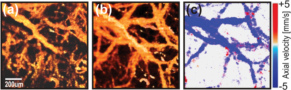

In the case of perpendicular flows, some qualitative assessment could be undertaken even in the absence of reasonable Doppler information. Blood motion, blood heterogeneities, and the chromatic effect¹¹ induce decreases in phase correlation between A-scans, causing high variability of the calculated mean Doppler shift. Because the variability of this noise is also valuable information, we also calculated the variance of mean Doppler shifts. Noise from bulk tissue differs from noise from flow areas because of different variance statistics, and it may also ensure angiographic contrast. In general, it is better to use speckle contrast to visualize flows that are perpendicular to the beam propagation. Figure 3 demonstrates clearly that reconstructed vascular is different in Fig. 3(a)–3(c) due to the differences of orientation of blood vessels. It is also implies that the Doppler variance can be slightly more sensitive [Fig. 4(b)] than the regular Doppler shift, but it still not very sensitive for perpendicular motion.

Note that, in the experiments presented, we did not take full advantage of the experimental setup with the resonant scanner. Careful analysis of the scanning beam trajectory shows that it is possible to receive two velocity ranges, thereby ensuring suitable oversampling. An OCT Doppler image can be generated either by taking spectral fringes with the same indexes within consecutive segments (as presented earlier in this paper) or by taking spectral fringes from within one segment. In the first case, oversampling is controlled by the oscillation amplitude of the $x$ galvo-scanner. The axial velocity range is provided by the resonant scanner period $T_{\text{segment}}$, which ensures a maximum measurable axial flow velocity value of $1\mathrm{mm}/\mathrm{s}$. In the second case, oversampling can be controlled by changing the oscillation amplitude of the resonant scanner. Because we are able to collect only 21 A-scans during one period of the resonant scanner, the oscillation amplitude should amount to several micrometers. Axial velocity range is provided by the camera repetition time $T_{\mathrm{rep}}$; thus, the maximal measurable axial flow velocity value is $21\mathrm{mm}/\mathrm{s}$. Since we have imaged the murine brain through the skull using the microscopic OCT system with limited depth of focus, we were able to observe only vessels in the cortical area very close to the skull. In this region, the orientation of the larger vessels is nearly perpendicular to the light beam, which results in a very small Doppler frequency shift. Otherwise, we would see the Doppler image of vessels in Fig. 3(c), which greatly exceeds the maximum detectable velocity. Therefore, we did not use all of the benefits of the setup, which can be applied to human retinal imaging.

To conclude, we have demonstrated the capability of STdOCT for 3-D study of blood flow in the brains of small animals through the intact skull. The modified OCT system and new scanning protocols were used to obtain both qualitative and quantitative information about vasculature from the same data set and from the same area of interest. The measurement time was also significantly shortened as a result of this method. We believe that further development of the proposed technique may provide a useful tool for biologists to study brain diseases and assess disease progression.