Applying a new computational method for biological tissue optics based on the time-dependent two-dimensional radiative transfer equation

Fatmir Asllanaj; Sebastien Fumeron

doi:10.1117/1.JBO.17.7.075007

9 July 2012 Applying a new computational method for biological tissue optics based on the time-dependent two-dimensional radiative transfer equation

Fatmir Asllanaj, Sebastien Fumeron

Author Affiliations +

Journal of Biomedical Optics, Vol. 17, Issue 7, 075007 (July 2012). https://doi.org/10.1117/1.JBO.17.7.075007

Abstract

Optical tomography is a medical imaging technique based on light propagation in the near infrared (NIR) part of the spectrum. We present a new way of predicting the short-pulsed NIR light propagation using a time-dependent two-dimensional-global radiative transfer equation in an absorbing and strongly anisotropically scattering medium. A cell-vertex finite-volume method is proposed for the discretization of the spatial domain. The closure relation based on the exponential scheme and linear interpolations was applied for the first time in the context of time-dependent radiative heat transfer problems. Details are given about the application of the original method on unstructured triangular meshes. The angular space (4ΠSr) is uniformly subdivided into discrete directions and a finite-differences discretization of the time domain is used. Numerical simulations for media with physical properties analogous to healthy and metastatic human liver subjected to a collimated short-pulsed NIR light are presented and discussed. As expected, discrepancies between the two kinds of tissues were found. In particular, the level of light flux was found to be weaker (inside the medium and at boundaries) in the healthy medium than in the metastatic one.

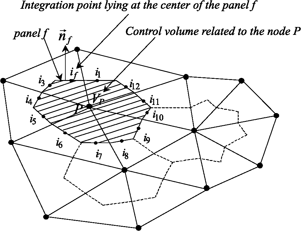
1. Introduction

The need to diagnose cancer tumors early, efficiently, and noninvasively has become a major public health issue. To this end, optical tomography (OT) is used to retrieve the thermo-optical properties of biological tissues with a radiative transfer model for visible or near infrared (NIR) light.¹^–³⁹ It consists in illuminating a tissue sample with a short-pulsed NIR light and then analyzing the information gathered to detect the possible presence of cancerous cells. Biological tissues scatter strongly, as cells are commonly made of many different structures (such as cores and mitochondria). Moreover, they absorb the infrared light because of their content in hemoglobin, melanin and water. Light can penetrate the tissues up to a depth of a few centimeters in a spectral range that is considered to be the therapeutic window (located between 600 and 900 nm), where the absorption of tissues is minimal.²⁹

In literature on the subject, diffusion approximation has commonly been used to model radiative transfer in biological tissues because of its mathematical simplicity and the availability of a vast amount of fast computational solvers. For example, in the paper by Schweiger et al.⁴⁰ a finite-element solution was used to solve the diffusion equation. The field of validity of the diffusion approximation was found to be relatively restricted because it is a low-order approximation which is only valid in the diffusion limit wherein scattering dominates absorption.³²^,³³ To overcome this problem, the time-dependent radiative transfer equation (TRTE) on short time scales,³²^,³³ or its Fourier space counterpart the frequency-domain radiative transfer equation (FD-RTE)¹²^,²⁰^,²³^,²⁷ can be used. In real applications, it should be noted that the time-dependent techniques (compared to the continuous and frequential techniques) offer the advantages of providing more informal and structural informations and a very high level of sensitivity. Thus, it seems more interesting to use the TRTE for modeling. For example, Jacques¹³ used a Monte-Carlo method to simulate the propagation of femtosecond and picosecond laser pulses within turbid tissues. Clearly, sufficiently accurate solution methods are required for OT while solving the TRTE or the FD-RTE in geometrically complex media and in the presence of anisotropically scattering it remains a challenging task.⁷^,²⁹ The Monte-Carlo statistical approach can be used to solve radiative transfer in biological tissues. This method is popular because it is accurate and simple to implement. However, it is highly expensive in terms of memory and computational time. Many other different solution methods have been developed to solve the radiative transfer equation in the spatial domain, including differential solution methods such as the Finite-Differences method (FDM), the finite-element method (FEM) and the finite-volume method (FVM). All these require the evaluation of the radiance at the cell faces of the control volumes that define the computational grid. Hence, the radiance at the cell faces has to be related to the radiance at the grid nodes (closure relations), which constitute the unknown factors of the discretized RTE. The STEP scheme, commonly referred to as upwind scheme in computation fluid dynamics (CFD), is only first-order accurate, and causes so-called false scattering (or numerical diffusion), whenever gradients of the radiance appear in directions not aligned with the direction of propagation of radiation.⁴¹^,⁴² False scattering can be sometimes reduced using grid refinement but this leads to a logical increase in computational time. Unlike the STEP scheme, the diamond scheme, which is the counterpart of the central difference scheme in CFD, is formally second-order accurate, but is not bounded. This means that physically unrealistic overshoots or undershoots, such as negative radiances, may appear in the numerical solution. Other more accurate schemes, such as the positive and exponential schemes, have been also proposed. The exponential scheme relies on the integral form of the RTE and was expected to be more precise than the STEP and diamond schemes. Other schemes still exist and we refer to Refs. 43–45 for more details. To our knowledge, the more precise spatial discretization schemes mentioned above have only been applied for steady state radiative heat transfer problems until now. We reviewed some studies on the computational methods for biological tissue optics. In the paper by Arridge and Schweiger³ photon transport models, such as the TRTE and the time-dependent diffusion equation, were described and methods for obtaining analytical and numerical solutions (FDM and FEM) for the most commonly used ones were reviewed but not detailed. In the paper by Klose and Hielscher⁴ an upwind (STEP) FDM was used to spatially solve the 2-D TRTE. The time discretization of the equation was carried out using a forward Euler differencing scheme. The article by Elaloufi et al.⁷ presents a study of the propagation of light pulses through participating media with anisotropic scattering based on the one-dimensional FD-RTE. A standard discrete-ordinate ( $S_{N}$ ) angular discretization was used to obtain a system of linear differential equations (one equation for each discrete direction used in the quadrature) and then a matrix eigenproblem approach was used to solve the system of differential equations. In papers by Rasmussen et al.²¹ coupled fluorescent RTE equations in frequency space were used to model excitation and emission light transport. The coupled equations were solved using the Attila transport software. Typically, the $S_{N}$ angular discretization was used and the equations were spatially solved using a robust linear discontinuous (LD) finite-element spatial differencing scheme. The method was applied to unstructured tetrahedral grids. In particular, the authors comparatively evaluated STEP differencing and linear discontinuous (LD) spatial differencing (used in the Attila package) on a phantom. They observed that the STEP differencing is a simple and inefficient scheme previously used in OT. Recently, a cell-center FVM with a second-order spatial differencing (diamond) scheme was used to solve the FD-RTE as presented in papers by Kim et al.²⁸^,³¹ The computational method was applied to three-dimensional (3-D) computational domains discretized with an unstructured tetrahedral mesh. Moreover, the works cited above sometimes go beyond solving the direct problem because they also implement the inverse problem in biological tissues. Difficulties related to false scattering (closure relations) in the numerical solution of the TRTE or the FD-RTE have been the subject of little discussion or study. The STEP and diamond schemes lead to errors, which are often quite serious. Our review of literature in this field shows they have been widely applied in OT, and are in fact sometimes still in use.

The objectives of the study covered in this paper are two-fold. The first objective was to present a cell-vertex (conservative) FVM on unstructured triangular meshes with an efficient closure relation based on an exponential scheme, which has yet to be used in time-dependent radiative heat transfer problems. The following section presents the problem statement and gives details of the computational method. The second objective was to apply the new computational method and then analyze and discuss the results for media with physical properties analog to healthy and metastatic human liver subjected to a collimated short-pulsed NIR light (850 nm). This is the subject of the third section. The last section reports our conclusions and suggests further developments for this work.

2. Numerical Treatment

2.1.

Problem Statement

Biological tissue is represented by a nongray participating medium with homogeneous optical properties (the wavelength is omitted in the notations for sake of simplicity). The effective medium is illuminated with a collimated short-pulsed light at normal incidence. Thus, a part of the pulsed collimated light beam leaves the medium without having been deviated, while the other fraction is scattered in multiple directions. The radiance inside the medium is made up of a $ψ_{c} (s, Ω, t)$ collimated component, which is the attenuated intensity of the collimated beam, as well as the $ψ_{c} (s, Ω, t)$ diffuse component, which is the in-scattered radiation into $Ω$ direction.⁴⁶ The intensity of the incoming pulse is $ϒ (t)$ , given at any location point $s_{w}$ on the bounding surface that is illuminated. Then, the $ψ_{c} (s, Ω, t)$ collimated radiation is governed by Bouguer-Beer-Lambert extinction law. From Appendix A, it follows that

Eq. (1)

ψ_{c} (s, Ω, t) = ϒ (t - \frac{n Δ_{s}}{c}) \exp (- μ_{t} Δ_{s}) δ (Ω - Ω_{c}) for t \geq \frac{n Δ_{s}}{c} and ψ_{c} (s, Ω, t) = 0 for t < \frac{n Δ_{s}}{c},

with

δ

the Dirac delta function,

Ω_{c}

the direction of the collimated radiation and,

Δ_{s}

the distance between points

s_{w}

and

s

. The

ψ (s, Ω, t)

diffuse radiation is solution of the TRTE with an additional radiative source term resulting from radiation scattered away from the collimated beam¹⁷^,¹⁸^,⁴¹^,⁴⁶

Eq. (2)

S_{c} (s, Ω, t) = μ_{s} p (Ω_{c} \to Ω) ϒ (t - \frac{n Δ_{s}}{c}) \exp (- μ_{t} Δ_{s}) .

The transient distribution $ϕ (s, t)$ and $Q_{in} (s, t)$ can be calculated respectively, as

Eq. (3)

ϕ (s, t) = \int_{4 π} ψ (s, Ω, t) + ψ_{c} (s, Ω, t) d Ω = \int_{4 π} ψ (s, Ω, t) d Ω + ϒ (t - \frac{n Δ_{s}}{c}) \exp (- μ_{t} Δ_{s}) Q_{in} (s, t) = \int_{n \cdot Ω < 0} ψ (s, Ω, t) | n \cdot Ω | d Ω [+ π ϒ (t - \frac{n Δ_{s}}{c}) \exp (- μ_{t} Δ_{s}) if n \cdot Ω_{c} < 0],

where the contribution of

ϒ

is valid only for

t \geq \frac{n Δ_{s}}{c}

.

2.2.

Discretization of the Time, Angular, and Spatial Domains

To solve the TRTE numerically on short time scales (typically going from 1 fs to 1 ps), the time domain was discretized with a $Δ t$ constant step such that $t_{k} = k Δ t, k \in {1, \dots, N_{t}}$ where $N_{t}$ was the necessary number of time steps to reach steady state (with a given precision). The angular space ( $4 π Sr$ ) was uniformly subdivided into $Ω^{(m, n)}$ discrete directions, $(m, n) \in {1, \dots, N_{θ}} \times {1, \dots, N_{φ}}$ $\in {1, . . ., N_{θ}} \times {1, . . ., N_{φ}}$ . Unstructured grids are generally seen to be superior to structured grids because they appear to be better at modeling arbitrarily shaped geometries. To work with 2-D irregular geometries, the computational spatial domain was divided into three-node triangular elements using unstructured meshes. In practice, we used a 2-D triangular mesh that generates three standard files giving: 1) the numbering and the coordinates of all the mesh’s nodes; 2) the numbering of triangles; 3) the numbering of elements (two nodes) at the boundary. The main advantage of this technique is the use of an automatic 2-D triangular mesh generator that would refine a zone of interest, for example the zone around an inclusion that would be present in the medium. In this work, a cell-vertex formulation was adopted. It consists in building control volumes around each node of the mesh and to compute the solution at the nodes of the mesh (nodes of triangles). The polygonal control volumes connected to each node were built by joining the centroids of the elements to the midpoints of the corresponding sides (Fig. 1). Control volumes surrounding the nodes at the boundaries were built as illustrated in. Ref. 47 All dependent variables were stored at the nodes of the grid. The surface of the control volume related to node $P$ was subdivided into $N_{f}$ surface elements. For a surface element $f$ , $i_{f}$ was the integration-point located at the center of surface element, $A_{f}$ was its surface area and, $n_{f}$ was the inward unit surface normal. It should be noted that the $i_{f}$ integration points of panels $f (f = 1, 2, \dots, 12)$ are defined only from the coordinates of the vertices of triangles of the mesh (Fig. 2). It is obvious that control volumes for a cell-vertex scheme applied to an unstructured triangular mesh are more difficult to implement. However, in our view, this should be more precise than cell-center schemes (for example) where the control volumes are defined by triangles and the unknowns are stored in the center of control volumes.²⁸^,³¹ Indeed, in our case the number of faces in a control volume was higher (Fig. 1) because it is equal to three for the cell-centre schemes.

Fig. 1

Control volume related to an interior node.

Fig. 2

Schematic of the problem. (a) Simplification of the geometry. (b) Problem geometry. (c) Gaussian pulse.

2.3.

Discretization of the TRTE

In general, the FVM gives a good accuracy computational time ratio (that is important for both forward and inverse problems). Moreover, unlike the FDM and the FEM, the FVM presents the advantage of being conservative. The total conservation of energy is ensured for each discrete component of the radiance, as for the radiative heat flux. Thus, the FVM ensures, for each component of the radiance, an exact radiative balance that increases the accuracy of the spatial discretization scheme. In addition, it was shown that with a sufficiently precise closure relation, this conservative method limits the problems of false scattering.⁴¹ In this context, we developed a modified FVM to simulate steady state radiative heat transfer problems.⁴⁷ The FVM implemented is a cell-vertex scheme (the solution is computed at the nodes of the mesh). The method was first applied to participating (nonscattering) gray media. In this section, we shall show that the method can be extended to time-dependent radiative heat transfer problems and for a scattering medium where the 2-D computational domain is discretized with unstructured triangular meshes.

2.3.1.

Explicit euler scheme and FVM applied to the TRTE

The integration of the TRTE over $V_{P}$ (Fig. 1) and into a $Δ Ω^{(m, n)}$ discrete solid angle centered around a $Ω^{(m, n)}$ discrete direction yields¹⁷^,¹⁸^,⁴¹

Eq. (4)

\int_{V_{P}} \int_{Δ Ω^{(m, n)}} \frac{n}{c} \frac{\partial ψ (s, Ω, t)}{\partial t} d Ω d V + \int_{V_{P}} \int_{Δ Ω^{(m, n)}} Ω \cdot \nabla ψ (s, Ω, t) d Ω d V + \int_{V_{P}} \int_{Δ Ω^{(m, n)}} μ_{t} ψ (s, Ω, t) d Ω d V = \int_{V_{P}} \int_{Δ Ω^{(m, n)}} S (s, Ω, t) d Ω d V + μ_{s} \int_{V_{P}} \int_{Δ Ω^{(m, n)}} \int_{Ω^{'} = 4 π} p (Ω^{'} \to Ω) ψ (s, Ω^{'}, t) d Ω^{'} d Ω d V,

where

ψ (s, Ω, t)

is the radiance defined at each point

s

of the medium, at time

t

and in a specific

Ω

direction of propagation of radiation. The source term is defined by

S (s, Ω, t) = n^{2} μ_{a} ψ_{b} [T (s, t)] + S_{c} (s, Ω, t)

. For a medium that is nonemitting,

S (s, Ω, t)

is reduced to

S_{c} (s, Ω, t)

. Inspection of Eq. (4) shows that, for isotropic scattering, the intensity field for

ψ

is readily determined from standard methods, after replacing

n^{2} μ_{a} ψ_{b} [T]

by

S

. In the case of anisotropic scattering the emission term

S

becomes direction-dependent, which may necessitate slight changes to the solution procedure.

By applying the divergence theorem to the second term of the left member of Eq. (4), it follows that

Eq. (5)

\int_{V_{P}} \int_{Δ Ω^{(m, n)}} Ω \cdot \nabla ψ (s, Ω, t) d Ω d V = \int_{Γ_{P}} \int_{Δ Ω^{(m, n)}} ψ (s, Ω, t) (Ω \cdot n_{ext}) d Ω d S .

Let $ψ_{i_{f}}^{k, (m, n)}$ be an approximation of the radiance at time $t_{k}$ , in the $i_{f}$ integration-point and in the $Ω^{(m, n)}$ discrete direction. Then, the relation Eq. (5) is approximated by

Eq. (6)

\sum_{f = 1}^{N_{f}} ψ_{i_{f}}^{k, (m, n)} A_{f} Δ_{f}^{(m, n)} with Δ_{f}^{(m, n)} = \int_{Δ Ω^{(m, n)}} Ω \cdot n_{f} d Ω .

It should be noted that $Δ_{f}^{(m, n)}$ is an integral that depends only on the orientation of surface element $f$ for the direction considered. This quantity is calculated in an exact way.⁴⁷ We assume that ( $ψ$ , $T$ ) and properties ( $μ_{a}$ , $μ_{s}$ ) are constant inside a sufficiently small $V_{P}$ control volume (taking only one value at node $P$ ) and inside $Δ Ω^{(m, n)}$ . If the explicit Euler (finite-difference) scheme is used for the time discretization of the TRTE, then the complete discretization of the Eq. (4) yields

Eq. (7)

\frac{n}{c} {\frac{ψ_{P}^{k + 1, (m, n)} - ψ_{P}^{k, (m, n)}}{Δ t}} Δ Ω^{(m, n)} V_{P} + \sum_{f = 1}^{N_{f}} ψ_{i_{f}}^{k, (m, n)} A_{f} Δ_{f}^{(m, n)} + μ_{t P} ψ_{P}^{k, (m, n)} Δ Ω^{(m, n)} V_{P} = {S_{P}^{k, (m, n)} + μ_{s P} \sum_{m^{'} = 1}^{N_{θ}} \sum_{n^{'} = 1}^{N_{φ}} {\tilde{P}}^{(m^{'}, n^{'}) \to (m, n)} ψ_{P}^{k, (m^{'}, n^{'})} Δ Ω^{(m^{'}, n^{'})}} Δ Ω^{(m, n)} V_{P} (m, n) \in {1, \dots, N_{θ}} \times {1, \dots, N_{φ}},

where

S_{P}^{k, (m, n)} = n^{2} μ_{a P} ψ_{b} [T_{P}^{k}] + S_{c, P}^{k, (m, n)}

with,

S_{c, P}^{k, (m, n)} = μ_{s P} {\tilde{p}}^{(m_{c}, n_{c}) \to (m, n)} ψ_{c} (P, Ω_{c}, t_{k}) \cdot {\tilde{p}}^{(m^{'}, n^{'}) \to (m, n)}

represents the average part of the scattered energy from the control solid angle

Δ Ω^{(m^{'}, n^{'})}

toward the control solid angle

Δ Ω^{(m, n)}

and is given by⁴⁸^,⁴⁹

Eq. (8)

{\tilde{p}}^{(m^{'}, n^{'}) \to (m, n)} = \frac{\int_{Δ Ω^{(m, n)}} \int_{Δ Ω^{(m^{'}, n^{'})}} p (Ω^{'} \to Ω) d Ω^{'} d Ω}{Δ Ω^{(m^{'}, n^{'})} Δ Ω^{(m, n)}} (m, n) \in {1, \dots, N_{θ}} \times {1, \dots, N_{φ}} and (m^{'}, n^{'}) \in {1, \dots, N_{θ}} \times {1, \dots, N_{φ}} .

2.3.2.

Spatial discretization of the transport term of the radiance

To solve the set of Eq. (7), closure relations between the $ψ_{i_{f}}^{k, (m, n)}$ integration-point values and the nodal values of the radiance are required. The directional nature of radiative transfer needed to be taken into account in order to establish the closure relations. Thus, for a specific direction of propagation of radiation, only the nodal values located upstream from the integration-point had to be considered. In our previous work,⁴⁷ original closure relations based on the exponential scheme and linear interpolations were developed to solve the steady state RTE. This technique was applied to a nonscattering gray medium with the same kind of mesh considered here for the computational spatial domain. We also tried the STEP and diamond schemes and opted to use the exponential scheme. The STEP scheme causes false diffusion that is a linear function of the spatial discretization. In case the grid point separation is sufficiently small (i.e., large mesh refinement), the impact of false diffusion becomes very small. The diamond scheme may yield oscillatory solutions. The exponential scheme relies on the integral form of the RTE and was expected to be more accurate than the other two schemes. It is however more expensive in terms of computational time. The results obtained verify the computational method and show the effectiveness of our closure relations, in particular for graded index media.⁵⁰ Our aim here was to generalize our closure relations to a scattering medium for the TRTE (the time has now to be taken into account) and in the case of an unstructured triangular mesh. It should be noted that the efficiency of the FVM in predicting radiative heat transfer in acute forward anisotropic scattering media illuminated with collimated radiation was recently shown in Ref. 49. In the same way as presented in Ref. 47, a locally rigorous one-dimensional (1-D) integration of the TRTE along the optical path ( $u_{f}$ , $i_{f}$ ) has to be used. Here, $u_{f}$ and $i_{f}$ are assumed to be on the same optical path of $Ω$ direction with $u_{f}$ located upstream from $i_{f}$ and $Δ_{s_{f}}$ is the distance between points $u_{f}$ and $i_{f}$ . From Appendix A, it follows

Eq. (9)

ψ (i_{f}, Ω, t) = ψ (u_{f}, Ω, t) \exp (- μ_{t} Δ_{s_{f}}) + \int_{u_{f}}^{i_{f}} {S (s, Ω, t) + μ_{s} \int_{Ω^{'} = 4 π} p (Ω^{'} \to Ω) ψ (s, Ω^{'}, t) d Ω^{'}} \exp [- μ_{t} (i_{f} - s)] d s .

It should be noted that it is difficult to evaluate the integral of Eq. (9) because $ψ (s, Ω^{'}, t)$ for $s \in (u_{f}, i_{f})$ is not known a priori. Thus, the following approximation can be used, $ψ (s, Ω^{'}, t) \approx ψ (u_{f}, Ω^{'}, t) s \in (u_{f}, i_{f})$ .

To compact the equations, the following notations are introduced where $a$ is the scattering albedo coefficient

Eq. (10)

D_{u_{f}}^{(m, n)} = A_{f} Δ_{f}^{(m, n)} \exp (- μ_{t} Δ_{s_{f}}); E_{u_{f}}^{(m, n)} = A_{f} Δ_{f}^{(m, n)} a [1 - \exp (- μ_{t} Δ_{s_{f}})] C_{u_{f}}^{k, (m, n)} = A_{f} Δ_{f}^{(m, n)} \int_{u_{f}}^{i_{f}} S^{k, (m, n)} (s) \exp [- μ_{t} (i_{f} - s)] d s .

Combining Eqs. (9) and (10) in Eq. (6) gives:

Eq. (11)

\sum_{f = 1}^{N_{f}} ψ_{i_{f}}^{k, (m, n)} A_{f} Δ_{f}^{(m, n)} = \sum_{f = 1}^{N_{f}} {ψ_{u_{f}}^{k, (m, n)} D_{u_{f}}^{(m, n)} + C_{u_{f}}^{k, (m, n)} + [\sum_{m^{'} = 1}^{N_{θ}} \sum_{n^{'} = 1}^{N_{φ}} {\tilde{p}}^{(m^{'}, n^{'}) \to (m, n)} ψ_{u_{f}}^{k, (m^{'}, n^{'})} Δ Ω^{(m^{'}, n^{'})}] E_{u_{f}}^{(m, n)}} .

The projections and linear interpolations presented in Ref. 47 were expected to improve the closure relations and the accuracy of the results. Also, they were used (and generalized) in this study, to link $ψ_{u_{f}}^{k, (m, n)}$ defined at the $u_{f}$ point with the nodal values of the radiance (see Appendix B). Combining Eqs. (7) and (11), the discretized TRTE gives the final expression

Eq. (12)

ψ_{P}^{k + 1, (m, n)} = ψ_{P}^{k, (m, n)} + Ψ [S_{P}^{k, (m, n)} - μ_{t P} ψ_{P}^{k, (m, n)} + μ_{s P} \sum_{m^{'} = 1}^{N_{θ}} \sum_{n^{'} = 1}^{N_{φ}} {\tilde{p}}^{(m^{'}, n^{'}) \to (m, n)} ψ_{P}^{k, (m^{'}, n^{'})} Δ Ω^{(m^{'}, n^{'})}] - Λ \sum_{f = 1}^{N_{f}} {ψ_{u_{f}}^{k, (m, n)} D_{u_{f}}^{(m, n)} + C_{u_{f}}^{k, (m, n)} + [\sum_{m^{'} = 1}^{N_{θ}} \sum_{n^{'} = 1}^{N_{φ}} {\tilde{p}}^{(m^{'}, n^{'}) \to (m, n)} ψ_{u_{f}}^{k, (m^{'}, n^{'})} Δ Ω^{(m^{'}, n^{'})}] E_{u_{f}}^{(m, n)}} (m, n) \in {1, \dots, N_{θ}} \times {1, \dots, N_{φ}},

with

Ψ = c Δ t / n

and

Λ = Ψ / Δ Ω^{(m, n)} V_{P}

. It has to be emphasized that the set of equations in Eq. (12) can only be solved for one given

(m, n)

direction. To evaluate double sums, it is necessary to know, as preliminary at time

t_{k}

, the specific intensities

ψ_{P}^{k, (m^{'}, n^{'})}

and

ψ_{u_{f}}^{k, (m^{'}, n^{'})}

in all discrete directions

(m^{'}, n^{'}) \in {1, \dots, N_{θ}} \times {1, \dots, N_{φ}}

. In our case, these specific intensities were changed by

ψ_{P}^{(k - 1), (m^{'}, n^{'})}

and

ψ_{u_{f}}^{(k - 1), (m^{'}, n^{'})}

, since the values are known at time

t_{k - 1}

. The convergence criterion to obtain a steady state solution was related to the values of the incoming radiative light fluxes calculated at the boundaries. Our computational method is designed to takes into account both opaque walls (with either purely specular or diffuse reflection), and semi-transparent walls (with reflecting or transmitting surface properties).

To the best of our knowledge, this is the first time that a cell-vertex FVM has been applied to solve the TRTE with the above closure relations established for unstructured triangular meshes. In order to test the efficiency (accuracy and stability) of our computational method, we examined benchmark cases (available in other works on similar topics) and found a good level of compliance. All the corresponding results are not presented here for the sake of conciseness. Only one benchmark is given in Appendix D to illustrate the performance of our computational method. All calculations presented were performed on an Intel Xeon E5540, 2.56 GHz with 12 Go RAM and using the intel FORTRAN compiler.

3. Results

3.1.

Model of Human Liver Subjected to Collimated Short-Pulsed NIR Light with Gaussian Profile

Experimentally, the tissue sample could be illuminated with a short-pulsed NIR light. As the sample is 3-D but the calculations are 2-D, we have to provide a $z$ -axis-independent fluence. This could be achieved by illuminating the sample with an extended line source along the $z$ -axis [Fig. 2(a)]. Along the $x$ -axis the light beam is collimated. In this study, the spatial width of the incident pulse is 1 mm on the surface of the sample, centered on the middle position [Fig. 2(b)]. A small section or tissue slice of the liver is represented by a rectangular cavity of dimension ( $1 mm \times 1 cm$ ) (1 mm according to the ( $O x$ )-axis) [Fig. 2(b)] with transparent boundaries. It should be noted that a medium, subjected to a collimated short-pulsed NIR radiation, can be treated as cold ( $T = 0 K$ ) because the blackbody emission intensity is always much smaller than the incident laser intensity; and is thus negligible. Then, the cavity studied is surrounded by a cold external medium ( $T = 0 K$ ). Each tissue is assumed to be nonemitting and its optical properties at 850 nm (NIR radiation) are taken from Table 1.

Table 1

Optical properties of healthy and metastatic human liver tissue (before thermal coagulation) at 850 nm.51

	Healthy liver	Metastatic liver
Absorption coefficient $μ_{a}$ ( ${mm}^{- 1}$ )	0.1	0.06
Scattering coefficient $μ_{s}$ ( ${mm}^{- 1}$ )	20.4	10.8
Asymmetry factor $g$	0.955	0.902
Optical penetration depth (mm)	1.8	2.3

It should be noted that it was not necessary to take a thickness larger than 1 mm since the optical penetration depth of the two tissues are of the order of a millimeter from Table 1. The two tissues are assumed to have the same refractive index, namely $n = 1.4$ , which is slightly higher than that of water.⁵² It should be noted that the absorption and scattering coefficients are both lower for the metastatic liver. In two cases, the medium is optically thick ( $τ = 20.5$ for healthy liver and $τ = 10.86$ for metastatic liver) and the regime of multiple scattering has to be considered ( $l_{s} ≪ L < l_{a}$ ). The Henyey-Greenstein phase function is used to account for the anisotropic nature of scattering by the medium and is expressed as: ⁴¹

Eq. (13)

p_{HG} (Θ) = \frac{1}{4 π} \frac{1 - g^{2}}{{[1 + g^{2} - 2 g \cos Θ]}^{3 / 2}} .

To solve the TRTE, the initial and boundary conditions need to be specified. Initially, at time $t = 0$ , there is no light (or photons) in the medium before light impingement. At subsequent times, the western wall of the medium is illuminated with a collimated short-pulsed beam at normal incidence (directed perpendicularly to the western wall) [Fig. 2(b)]. The incident radiation is assumed to be Gaussian with a peak intensity $I_{0}$ at time $t = t_{c}$ and pulse width $t_{p}$ [Fig. 2(c)]. The intensity profile for a Gaussian beam, which is commonly used, can be expressed as²⁴^,⁴⁶

Eq. (14)

ϒ (t) = I_{0} \exp [- 4 \ln 2 {(\frac{t - t_{c}}{t_{p}})}^{2}], 0 < t < 2 t_{c} and ϒ (t) = 0, t \geq 2 t_{c} .

The selected pulse width $t_{p}$ was 0.1 ps, $t_{c} / t_{p} = 1.5$ , and $I_{0} = 10 W m^{- 2}$ . The intensity is typical of a collimated beam from a pulsed LED with a peak power of 1 mW shining on an area of about $1 {cm}^{2}$ . Our simulations were carried out with a structured triangular mesh composed of ( $50 \times 250$ ) nodes (50 according to the ( $O x$ )-axis). To correctly take into account the first scattering events in the tissue ( $l_{s} = 0.049 mm$ for healthy liver and $l_{s} = 0.092 mm$ for metastatic liver), the grid was refined near to the west face of the medium, according to the ( $O x$ )-axis and a geometric progression with a ratio equal to 0.95. Thus, the first node of the grid was 0.009 mm from the west face of the medium. The angular space was subdivided into $N_{θ} \times N_{φ} = 64 \times 32$ control solid angles. The Courant-Friedrich-Levy (CFL) condition⁶^,¹⁷ was satisfied in our calculations, $Δ t \leq \frac{n}{c} Δ s_{\min}$ where $Δ s_{\min}$ is the size of the smallest cell. In other words, the traveling distance of a ray of light between two consecutive time steps does not exceed the size of the smallest cell. In our case, $Δ s_{\min} = 0.009 mm$ and $\frac{n}{c} Δ s_{\min} = 0.041 ps$ . Thus, $Δ t$ was chosen to be 0.01 ps and the Crank Nicolson scheme was used for the time discretization of the TRTE (see Appendix C). Furthermore, sensitivity studies have been carried out on time, spatial and angular discretizations and the values chosen show that the grid influence remained weak. Under the conditions specified above, the computational time required by our program to carry out 600 time steps was about 115 h.

3.2.

Results and Discussion

The numerical results obtained for the Gaussian pulse reveal several important points. The radiative flux reaching the different boundaries is shown in Figs. 3 and 4 and radiative flux inside the biological medium (metastatic and healthy) is depicted in Figs. 5 and 6. As expected, discrepancies appeared between the two kinds of tissues appear. At each time step, the light flux was weaker (inside the medium and at boundaries) in the healthy medium than in the metastatic one. As explained previously, this comes from the fact that absorption coefficient is greater in healthy tissue ( $0.1 {mm}^{- 1}$ against $0.06 {mm}^{- 1}$ for metastatic liver). It appears that radiative flux undergoes an important extinction during its propagation in the tissue: at $x = 0.2 mm$ of the sample, the beam has lost more than $45 %$ of its power (Fig. 6). Moreover, it is simple to check that the pulse peak propagates at $\frac{D x}{D t} = \frac{0.2 - 0.1}{1.13 - 0.66} 1 0^{9} \approx 2.1 1 0^{8}$ , which is of the order of the phase velocity $c / n$ (assumed identical to group velocity for a constant refractive index $n = 1.4$ ). Just before leaving the medium, levels of light flux impinging on the east face are represented. The dimensionless power density was about $2.5 1 0^{- 10}$ for healthy tissue and about $6 1 0^{- 6}$ for metastatic tissue (Fig. 4). This discrepancy is helpful when comparing the respective weight of absorption and scattering processes. Biological media are considered to be strongly scattering. Here, the absorption coefficient, scattering coefficient (twice that of metastatic liver) and asymmetry factor of a healthy liver were all found to be stronger than those of a metastatic liver. If scattering prevailed over absorption, then as scattering is favored forward, incoming light flux on the east side should be greater for healthy liver compared to metastatic liver. Figure 4 shows the contrary, meaning that absorption has to prevail over scattering. Moreover, as the levels of light flux impinging on the east face are extremely low, this means that for medical imaging applications, transmitted light flux could hardly be measurable. Therefore, it seems more relevant to focus on the backscattered light flux (Fig. 3). For metastatic tissue, dimensionless backscattered light flux is about $2 1 0^{- 3}$ , just a little higher than that obtained for healthy tissues. The absolute difference varies between 0 and $0.8 1 0^{- 3}$ . Therefore to efficiently discriminate between both kinds of media would require further information, such as the state of polarization or the implementation of more refined models, to obtain qualitative differences in the behavior of tissues with respect to a short-pulsed NIR light.

Fig. 3

Evolution of dimensionless incoming radiative flux in the middle position of the west face (reflectance).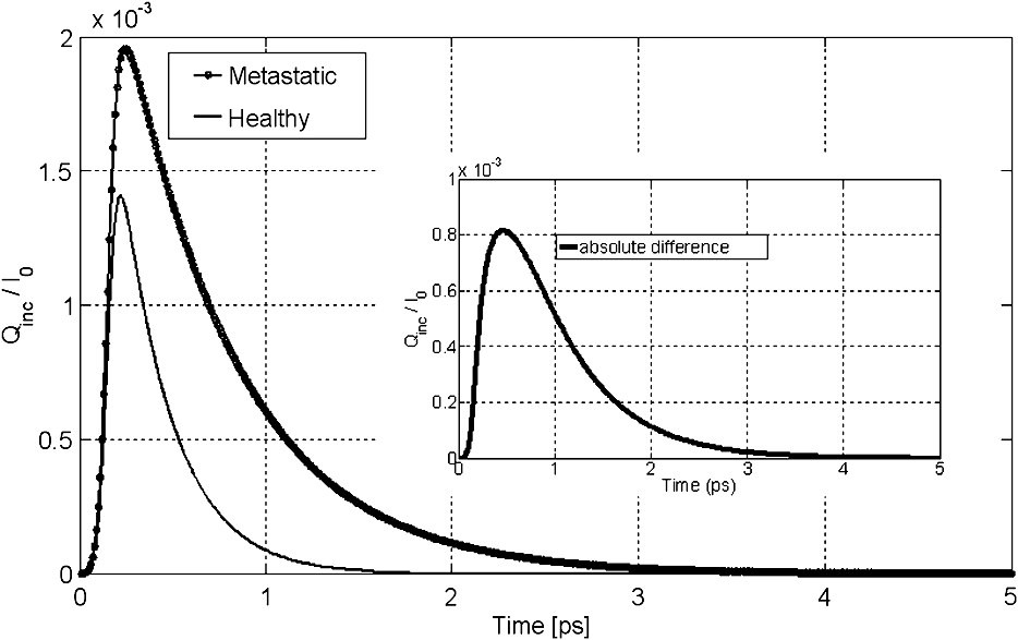

Fig. 4

Dimensionless incoming radiative flux on the East face at different times (transmittance). (a) Healthy tissue. (b) Metastatic tissue.

Fig. 5

Evolution of dimensionless radiative flux (diffuse component) along the ( $O x$ ) axis in the medium. (a) Healthy tissue. (b) Metastatic tissue.

Fig. 6

Evolution of dimensionless radiative flux (diffuse component) in the middle position of the medium along the ( $O x$ ) axis.

Finally, diffuse radiative flux gives a luminous halo around the collimated light, that increases versus time (Fig. 5). Whereas the spatial width of the incident pulse is 1 mm on the west surface of the sample, diffuse radiative flux is extended on approximately 2 mm on the east surface of the sample (Fig. 4).

4. Conclusion

This paper presents a new solution method for the TRTE in 2-D absorbing an strongly anisotropically scattering medium subjected to a collimated short-pulsed NIR light. A cell-vertex FVM was proposed for the discretization of the spatial domain. The closure relation based on the exponential scheme and linear interpolations was applied for the first time in the context of time-dependent radiative heat transfer problems. Details were given about the application of the original method on unstructured triangular meshes. A finite-differences discretization of the time domain was used. The developed code was tested with some benchmark cases (through comparisons with existing published solutions) and was found to be robust, stable and accurate.

Numerical simulations for media with physical properties analog to healthy and metastatic human liver subjected to a collimated short-pulsed NIR light were presented and discussed. The propagation speed of light pulse inside the medium is reproduced correctly. As expected, discrepancies between the two kinds of tissues were observed. Indeed, at each time step the level of light flux was found to be weaker (inside the medium and at boundaries) in the healthy medium than in the metastatic one. Moreover, our results indicate that the dominant mechanism for extinction of light in liver was absorption, which suggests the possibility of tumoral diagnostics based on recomposition of the absorption field.

In OT, it is very useful to have efficient numerical schemes and closures relations to reduce false scattering in the TRTE model. In our future work, we will aim to provide relevant comparative analyses between different schemes, such as step, diamond, mean flux, exponential, cell-center formulation and others found in articles on this subject. To evaluate in an objective way the efficiency of the present computational method in terms of precision and computational time, it would be interesting to carry out comparisons with other existing radiative transfer methods, including Monte-Carlo methods on benchmark cases in the same configurations (angular, spatial and temporal grids).

To develop an efficient tool for cancer tumoral diagnostic it is clear from our results that this work could usefully be extended to include other properties of light beams to discriminate between healthy and metastatic tissues. For example, our work was limited to unpolarized light, but laser sources can also be polarized (circularly or linearly). Thus, states of polarization for the specific radiance (based on the vector radiative transfer equation) together with specular reflections may result in a number of interesting effects and could be implemented by using the Stokes formalism.⁵³^–⁵⁵

Other improvements can also be made to the thermo-optical model of the biological medium. Only homogeneous media with constant optical properties were considered here and for the metastatic case: this implies the presence of a developed tumor that fills the whole simulation domain. With the aim of achieving early diagnosis of the presence of tumors, a more relevant approach would be to consider a healthy tissue inside which a tumor may exist as a small inclusion. This would involve space-varying thermo-optical properties and internal boundaries.

Another possible development is to take into account the disordered nature of biological tissues. Several works have already underlined the turbulent nature of the optical properties’s variations in biological tissues.⁵⁶ Taking into account random spatial variations for the refractive index leads to both coherent and incoherent scattering, whereas random spatial variations of the absorption coefficient can result in bleaching.⁵⁷ Both features may be of prime importance for OT.

Appendices

Appendix A:

Integral Formulation of the TRTE

The integral formulation of the TRTE along the optical path $(u_{f}, i_{f})$ is ⁵⁸

Eq. (15)

ψ (i_{f}, Ω, t) = ψ (u_{f}, Ω, γ (t)) \exp (- μ_{t} Δ_{s_{f}}) + \int_{u_{f}}^{i_{f}} {S (s, Ω, ζ (t)) + μ_{s} \int_{Ω^{'} = 4 π} p (Ω^{'} \to Ω) ψ (s, Ω^{'}, ζ (t)) d Ω^{'}} \exp (- μ_{t} (i_{f} - s)) d s,

with

γ (t) = t - \frac{n Δ_{s_{f}}}{c}

and

ζ (t) = t - \frac{n (i_{f} - s)}{c}

. Equation (15) is valid for

γ (t) \geq 0

and

ψ (i_{f}, Ω, t) = 0

for

γ (t) < 0

. It should be noted that with the CFL condition,

γ (t) \leq t - Δ t

and

ζ (t) \leq t - Δ t

. Also, it should be noted that in the integral,

S (s, Ω, ζ (t))

and

ψ (s, Ω^{'}, ζ (t))

for

s \in (u_{f}, i_{f})

are not known a priori. To simplify the calculations, the terms at time

γ (t)

and

ζ (t)

can be approximated by these same terms at time

t

. This approximation is justified if the length of the optical path

Δ_{s_{f}}

is extremely short, which is the case for sufficiently small control volumes. Thus, the integral formulation of the TRTE is reduced to the integral formulation of the steady state RTE.⁴¹

Appendix B:

Projections and Linear Interpolations

To simplify, a notation was introduced: $A < = B$ means point $A$ is upstream from point $B$ . A $Ω$ specific direction of radiation and a triangle of reference denoted by $J = (P_{1}, P_{2}, P_{3})$ with $P_{1} < = P_{2} < = P_{3}$ are considered (Fig. 7). $Δ P_{l} (l = 1, 2, 3)$ are the planes orthogonal to the $Ω$ direction and that pass respectively by $P_{l}$ . The $i_{l} (l = 1, 2, 3)$ integration points are related to the $J$ triangle.

Fig. 7

Projection of integration points $i_{f}$ ( $f = 1$ , 2, 3) in a $Ω$ specific direction and a $(P_{1}, P_{2}, P_{3})$ triangle of reference.

For cases presented further, except in particular cases such as boundaries (see Ref. 47 for the details), points $u_{1}$ and $u_{2}$ are always built in the same way. The $i_{f}$ ( $f = 1, 2$ ) integration points are projected on lines perpendicular to the $Ω$ direction and located upstream from points $i_{1}$ and $i_{2}$ , the line $Δ P_{1}$ in the case of points $u_{1}$ and $u_{2}$ (Fig. 7). The point $u_{3}$ is the intersection point, located upstream from $i_{3}$ , between the $Ω$ direction and the first side met of an element of $J$ . Thus, only two cases can arise: $u_{3}$ is on the line $(P_{1}, P_{2})$ or, it is on the line $(P_{1}, P_{3})$ . In our case, radiances at points $u_{f}$ are approximated by linear interpolation with the values of the closest upstream nodes. Thus, the following principal relations have to be taken into account

Eq. (16)

ψ_{u_{1}}^{(m, n)} \approx ψ_{P_{1}}^{(m, n)}; ψ_{u_{2}}^{(m, n)} \approx ψ_{P_{1}}^{(m, n)} (m, n) \in {1, \dots, N_{θ}} \times {1, \dots, N_{φ}} .

If $u_{3}$ is on the line $(P_{1}, P_{2})$ or on the line $(P_{1}, P_{3})$ , one has

Eq. (17)

ψ_{u_{3}}^{(m, n)} \approx \frac{| u_{3} P_{2} |}{| u_{3} P_{1} | + | u_{3} P_{2} |} ψ_{P_{1}}^{(m, n)} + \frac{| u_{3} P_{1} |}{| u_{3} P_{1} | + | u_{3} P_{2} |} ψ_{P_{2}}^{(m, n)} (m, n) \in {1, \dots, N_{θ}} \times {1, \dots, N_{φ}} .

In the same way, the double sum in Eq. (11) (related to the scattering) is approximated by

Eq. (18)

\sum_{m^{'} = 1}^{N_{θ}} \sum_{n^{'} = 1}^{N_{φ}} {\tilde{p}}^{(m^{'}, n^{'}, m, n)} ψ_{u_{l}}^{(m^{'}, n^{'})} Δ Ω^{(m^{'}, n^{'})} \approx \sum_{m^{'} = 1}^{N_{θ}} \sum_{n^{'} = 1}^{N_{φ}} {\tilde{p}}^{(m^{'}, n^{'}, m, n)} ψ_{P_{l}}^{(m^{'}, n^{'})} Δ Ω^{(m^{'}, n^{'})} (l = 1, 2), \sum_{m^{'} = 1}^{N_{θ}} \sum_{n^{'} = 1}^{N_{φ}} {\tilde{p}}^{(m^{'}, n^{'}, m, n)} ψ_{u_{3}}^{(m^{'}, n^{'})} Δ Ω^{(m^{'}, n^{'})}

Eq. (19)

\approx \sum_{m^{'} = 1}^{N_{θ}} \sum_{n^{'} = 1}^{N_{φ}} {\tilde{p}}^{(m^{'}, n^{'}, m, n)} {\frac{| u_{3} P_{2} |}{| u_{3} P_{1} | + | u_{3} P_{2} |} ψ_{P_{1}}^{(m^{'}, n^{'})} + \frac{| u_{3} P_{1} |}{| u_{3} P_{1} | + | u_{3} P_{2} |} ψ_{P_{2}}^{(m^{'}, n^{'})}} Δ Ω^{(m^{'}, n^{'})}, (m, n) \in {1, \dots, N_{θ}} \times {1, \dots, N_{φ}} .

It should be noted that node $P_{3}$ was not considered in the formula since, by construction (Fig. 7), it is located downstream from the $i_{f} (f = 1, 2, 3)$ integration points. For particular cases, we invite the reader to refer to Ref. 47 for the details.

Appendix C:

$α$ -Scheme Applied to the TRTE

The precision in time of the computational scheme Eq. (12) can be improved by using the well-known $α$ -scheme with $0 \leq α \leq 1$ . Let us recall that $α = 0; 0.5; 1$ correspond respectively to the explicit, Crank-Nicolson and implicit schemes. In our case, the $α$ -scheme is written as

Eq. (20)

ψ_{P}^{k + 1, (m, n)} - α Ψ [S_{P}^{k + 1, (m, n)} - μ_{t P} ψ_{P}^{k + 1, (m, n)} + μ_{s_{P}} \sum_{m^{'} = 1}^{N_{θ}} \sum_{n^{'} = 1}^{N_{φ}} {\tilde{p}}^{(m^{'}, n^{'}) \to (m, n)} ψ_{P}^{k + 1, (m^{'}, n^{'})} Δ Ω^{(m^{'}, n^{'})}] + α Λ \sum_{f = 1}^{N_{f}} {ψ_{u_{f}}^{k + 1, (m, n)} D_{u_{f}}^{(m, n)} + C_{u_{f}}^{k + 1, (m, n)} + [\sum_{m^{'} = 1}^{N_{θ}} \sum_{n^{'} = 1}^{N_{φ}} {\tilde{p}}^{(m^{'}, n^{'}) \to (m, n)} ψ_{u_{f}}^{k + 1, (m^{'}, n^{'})} Δ Ω^{(m^{'}, n^{'})}] E_{u_{f}}^{(m, n)}} = ψ_{P}^{k, (m, n)} + (1 - α) Ψ [S_{P}^{k, (m, n)} - μ_{t P} ψ_{P}^{k, (m, n)} + μ_{s_{P}} \sum_{m^{'} = 1}^{N_{θ}} \sum_{n^{'} = 1}^{N_{φ}} {\tilde{p}}^{(m^{'}, n^{'}) \to (m, n)} ψ_{P}^{k, (m^{'}, n^{'})} Δ Ω^{(m^{'}, n^{'})}] - (1 - α) Λ \sum_{f = 1}^{N_{f}} {ψ_{u_{f}}^{k, (m, n)} D_{u_{f}}^{(m, n)} + C_{u_{f}}^{k, (m, n)} + [\sum_{m^{'} = 1}^{N_{θ}} \sum_{n^{'} = 1}^{N_{φ}} {\tilde{p}}^{(m^{'}, n^{'}) \to (m, n)} ψ_{u_{f}}^{k, (m^{'}, n^{'})} Δ Ω^{(m^{'}, n^{'})}] E_{u_{f}}^{(m, n)}} (m, n) \in {1, \dots, N_{θ}} \times {1, \dots, N_{φ}] .

It should be noted that if the medium is assumed to be emitting and if temperature is not constant inside the medium then, a development in Taylor series at the first-order can be used to evaluate the term $ψ_{b} [T_{P}^{k + 1}]$ at time $t_{k + 1}$

Eq. (21)

ψ_{b} [T_{P}^{k + 1}] = ψ_{b} [T_{P}^{k}] + (T_{P}^{k + 1} - T_{P}^{k}) \frac{d ψ_{b} [T]}{d T} (T^{k}) .

Appendix D:

Verification of the Computational Method

To verify the accuracy and stability of the computational method for solving transient radiative transfer problem in our context, a benchmark case closest to our application was examined. An absorbing and anisotropically scattering medium in square cavity of length $L^{*} = 10$ with transparent walls was considered. The left face was subjected to collimated short-pulsed light with square profile (the pulse width $t_{p}^{*} = 1$ ) having a peak intensity of unit magnitude. The scattering albedo was equal to 0.998 and the scattering phase function considered was of linear anisotropic form: $p (Θ) = 1 + ρ \cos Θ$ . Positive and negative values of the coefficient $ρ$ correspond to forward and backward scattering phase function, respectively. The effect of anisotropic scattering on the transient transmittance and reflectance at the central position of the east and west faces of the medium respectively are presented (Fig. 8). A comparison between our results and numerical solutions obtained by Sakami et al.⁸ are given. In Ref. 8, a FDM with a high order upwind piecewise parabolic interpolation scheme (known in CFD) was used to spatially solve the TRTE. The $S_{8}$ angular discretization and a fully implicit scheme to discretize the transient term were performed. To facilitate the comparison, we used angular and spatial discretizations close to those selected by the authors. A good level of compliance was found and the few small differences observed can be attributed to the completely different computational methods that were used. Under the conditions specified above, the computational time required by our program to carry out 2,000 time steps ( $Δ t^{*} = 0.05$ ) was about 86 min.

Fig. 8

Effect of anisotropic scattering on the transient transmittance and reflectance. (a) Transmittance—Present study. (b) Transmittance⁸. (c) Reflectance—Present study. (d) Reflectance⁸

References

1.

J. C. HebdenS. R. ArridgeD. T. Delpy, “Optical imaging in medicine: I. experimental techniques,” Phys. Med. Biol., 42 (5), 825 –840 (1997). http://dx.doi.org/10.1088/0031-9155/42/5/007 PHMBA7 0031-9155 Google Scholar

2.

S. R. ArridgeJ. C. Hebden, “Optical imaging in medicine: II. modelling and reconstruction,” Phys. Med. Biol., 42 (5), 841 –853 (1997). http://dx.doi.org/10.1088/0031-9155/42/5/008 PHMBA7 0031-9155 Google Scholar

3.

S. R. ArridgeM. Schweiger, “Image reconstruction in optical tomography,” Phil. Trans. R Soc. Lond. B, 352 (1354), 717 –726 (1997). http://dx.doi.org/10.1098/rstb.1997.0054 0962-8436 Google Scholar

4.

A. D. KloseA. H. Hielscher, “Iterative reconstruction scheme for optical tomography based on the equation of radiative transfer,” Med. Phys., 26 (8), 1698 –1707 (1999). http://dx.doi.org/10.1118/1.598661 MPHYA6 0094-2405 Google Scholar

5.

S. R. Arridge, “Optical tomography in medical imaging,” Topical Review. Inv. P, 15 (2), R41 –R93 (1999). Google Scholar

6.

Z. GuoS. Kumar, “Discrete-ordinates solution of short-pulsed laser transport in two-dimensional turbid media,” Appl. Opt., 40 (19), 3156 –3163 (2001). http://dx.doi.org/10.1364/AO.40.003156 APOPAI 0003-6935 Google Scholar

7.

R. ElaloufiR. CarminatiJ. J. Greffet, “Time-dependent transport through scattering media: from radiative transfer to diffusion,” J. Opt. A Pure Appl. Opt., 4 (5), S103 –S108 (2002). http://dx.doi.org/10.1088/1464-4258/4/5/355 1464-4258 Google Scholar

8.

M. SakamiK. MitraP. F. Hsu, “Analysis of light pulse transport through two-dimensional scattering and absorbing media,” J. Quant. Spectrosc. Radiat. Transfer, 73 (2–5), 169 –179 (2002). http://dx.doi.org/10.1016/S0022-4073(01)00216-3 JQSRAE 0022-4073 Google Scholar

9.

A. D. Kloseet al., “Optical tomography using the time independent equation of radiative transfer. part1: forward model,” J. Quant. Spectrosc. Radiat. Transfer, 72 (5), 691 –713 (2002). http://dx.doi.org/10.1016/S0022-4073(01)00150-9 JQSRAE 0022-4073 Google Scholar

10.

A. D. KloseA. H. Hielscher, “Optical tomography using the time independent equation of radiative transfer. part2: inverse model,” J. Quant. Spectrosc. Radiat. Transfer, 72 (5), 715 –732 (2002). http://dx.doi.org/10.1016/S0022-4073(01)00151-0 JQSRAE 0022-4073 Google Scholar

11.

G. AbdoulaevA. H. Hielscher, “Three-dimensional optical tomography with the equation of radiative transfer,” J. Elect. Imag., 12 (4), 594 –60 (2003). http://dx.doi.org/10.1117/1.1587730 1017-9909 Google Scholar

12.

K. Renet al., “Algorithm for solving the equation of radiative transfer in the frequency domain,” Opt. Lett., 29 (6), 578 –580 (2004). http://dx.doi.org/10.1364/OL.29.000578 OPLEDP 0146-9592 Google Scholar

13.

S. L. Jacques, “Time resolved propagation of ultrashort laser pulses within turbid tissues,” Appl. Opt., 28 (12), 2223 –2229 (1989). http://dx.doi.org/10.1364/AO.28.002223 APOPAI 0003-6935 Google Scholar

14.

A. P. GibsonJ. C. HebdenS. R. Arridge, “Recent advances in diffuse optical imaging,” Phys. Med. Biol., 50 (4), R1 –R43 (2005). http://dx.doi.org/10.1088/0031-9155/50/4/R01 PHMBA7 0031-9155 Google Scholar

15.

T. Tarvainenet al., “Coupled radiative transfer equation and diffusion approximation model for photon migration in turbid medium with low-scattering and non-scattering regions,” Phys. Med. Biol., 50 (20), 4913 –4930 (2005). http://dx.doi.org/10.1088/0031-9155/50/20/011 PHMBA7 0031-9155 Google Scholar

16.

T. Tarvainenet al., “Hybrid radiative-transfer-diffusion model for optical tomography,” Appl. Opt., 44 (6), 876 –886 (2005). http://dx.doi.org/10.1364/AO.44.000876 APOPAI 0003-6935 Google Scholar

17.

J. BoulangerA. Charette, “Numerical developments for short-pulsed near infra-red laser spectroscopy. part I: direct treatment,” J. Quant. Spectrosc. Radiat. Transfer, 91 (2), 189 –209 (2005). http://dx.doi.org/10.1016/j.jqsrt.2004.05.057 JQSRAE 0022-4073 Google Scholar

18.

J. BoulangerA. Charette, “Numerical developments for short-pulsed near infra-red laser spectroscopy. part II: inverse treatment,” J. Quant. Spectrosc. Radiat. Transfer, 91 (3), 297 –318 (2005). http://dx.doi.org/10.1016/j.jqsrt.2004.05.062 JQSRAE 0022-4073 Google Scholar

19.

S. R. Arridgeet al., “Reconstruction of subdomain boundaries of piecewise constant coefficients of the radiative transport equation from optical tomography data,” Inverse Probl., 22 (6), 2175 –2198 (2006). Google Scholar

20.

K. Renet al., “Frequency-domain optical tomography based on the equation of radiative transfer,” Siam. J. Sci. Comp., 28 (4), 1463 –1489 (2006). http://dx.doi.org/10.1137/040619193 1064-8275 Google Scholar

21.

J. C. Rasmussenet al., “Radiative transport in fluorescence-enhanced frequency domain photon migration,” Med. Phys., 33 (12), 4685 –4700 (2006). http://dx.doi.org/10.1118/1.2388572 MPHYA6 0094-2405 Google Scholar

22.

V. V. Tuchin, Tissue Optics: Light Scattering Methods and Instruments for Medical Diagnosis, 2nd ed.SPIE Press, Washington, Bellingham (2007). Google Scholar

23.

X. GuK. RenA. H. Hielscher, “Frequency-domain sensitivity analysis for small imaging domains using the equation of radiative transfer,” Appl. Opt., 46 (10), 1624 –1632 (2007). http://dx.doi.org/10.1364/AO.46.001624 APOPAI 0003-6935 Google Scholar

24.

K. D. SmithK. M. KatikaL. Pilon, “Maximum time-resolved hemispherical reflectance of absorbing and isotropically scattering media,” J. Quant. Spectrosc. Radiat. Transfer, 104 (3), 384 –399 (2007). http://dx.doi.org/10.1016/j.jqsrt.2006.09.008 JQSRAE 0022-4073 Google Scholar

25.

A. CharetteJ. BoulangerH. K. Kim, “An overview on recent radiation transport algorithm development for optical tomography imaging,” J. Quant. Spectrosc. Radiat. Transfer, 109 (17–18), 2743 –2766 (2008). http://dx.doi.org/10.1016/j.jqsrt.2008.06.007 JQSRAE 0022-4073 Google Scholar

26.

A. D. KloseA. H. Hielscher, “Optical tomography with the equation of radiative transfer,” Int. J. Num. Meth. Heat Fluid Flow, 18 (3–4), 443 –464 (2008). http://dx.doi.org/10.1108/09615530810853673 0961-5539 Google Scholar

27.

T. TarvainenM. VaukhonenS.R. Arridge, “Gauss-newton reconstruction method for optical tomography using the finite element solution of the radiative transfer equation,” J. Quant. Spectrosc. Radiat. Transfer, 109 (17–18), 2767 –2778 (2008). http://dx.doi.org/10.1016/j.jqsrt.2008.08.006 JQSRAE 0022-4073 Google Scholar

28.

H. K. Kimet al., “Optimal source-modulation frequencies for transport theory based optical tomography of small-tissue volumes,” Opt. Express, 16 (22), 18082 –18101 (2008). http://dx.doi.org/10.1364/OE.16.018082 OPEXFF 1094-4087 Google Scholar

29.

AD. Klose, “Light Scattering” in Radiative Transfer of Luminescence Light in Biological Tissue, 293 –345 Springer, Berlin, Germany (2009). Google Scholar

30.

S. R. ArridgeJ. C. Schotland, “Optical tomography: forward and inverse problems,” Inverse Probl., 25 (12), 123010 (2009). Google Scholar

31.

H. K. KimA. H. Hielscher, “A PDE-constrained SQP algorithm for optical tomography based on the frequency-domain equation of radiative transfer,” Inverse Probl., 25 (1), 015010 (2009). Google Scholar

32.

A. D. Klose, “The forward and inverse problem in tissue optics based on the radiative transfer equation: a brief review,” J. Quant. Spectrosc. Radiat. Transfer, 111 (11), 1852 –1853 (2010). http://dx.doi.org/10.1016/j.jqsrt.2010.01.020 JQSRAE 0022-4073 Google Scholar

33.

F. Martelliet al., Light Propagation Through Biological Tissue and Other Diffusive Media: Theory, Solutions, and Software, SPIE Press, Washington, Bellingham (2010). Google Scholar

34.

L. D. MontejoA. D. KloseA. H. Hielscher, “Implementation of the equation of radiative transfer on block-structured grids for modeling light propagation in tissue,” Biomed. Opt. Exp., 1 (3), 861 –878 (2010). http://dx.doi.org/10.1364/BOE.1.000861 BOEICL 2156-7085 Google Scholar

35.

T. Tarvainen, “An approximation error approach for compensating for modelling errors between the radiative transfer equation and the diffusion approximation in diffuse optical tomography,” Inv. P., 26 (1), 015005 (2010). Google Scholar

36.

H. K. Kimet al., “Hielscher PDE-constrained multispectral imaging of tissue chromophores with the equation of radiative transfer,” Biomed. Opt. Exp., 1 (3), 812 –824 (2010). http://dx.doi.org/10.1364/BOE.1.000812 JBOPFO 1083-3668 Google Scholar

37.

P. S. Mohanet al., “Variable order spherical harmonic expansion scheme for the radiative transport equation using finite elements,” J. Comp. Phys., 230 (19), 7364 –7383 (2011). http://dx.doi.org/10.1016/j.jcp.2011.06.004 JCTPAH 0021-9991 Google Scholar

38.

T. Tarvainenet al., “Image reconstruction in diffuse optical tomography using the coupled radiative transport—diffusion model,” J. Quant. Spectrosc. Radiat. Transfer, 112 (16), 2600 –2608 (2011). http://dx.doi.org/10.1016/j.jqsrt.2011.07.008 JQSRAE 0022-4073 Google Scholar

39.

PilonL.KatikaK. M., “Time-resolved non-invasive optometric device for medical diagnostic,” U. S. Patent No. 7,904,140 B2 (2011).

40.

M. SchweigerS. R. ArridgeD. T. Delpy, “Application of the finite-element method for the forward and inverse models in optical tomography,” J. Math. Imag. Vis., 3 (3), 263 –283 (1993). http://dx.doi.org/10.1007/BF01248356 0924-9907 Google Scholar

41.

M. Modest, Radiative Heat Transfer, 2nd ed.Academic Press, San Diego, CA (2003). Google Scholar

42.

PJ. Coelho, “The role of ray effects and false scattering on the accuracy of the standard and modified discrete ordinates methods,” J. Quant. Spectrosc. Radiat. Transfer, 73 (2–5), 231 –238 (2002). http://dx.doi.org/10.1016/S0022-4073(01)00202-3 JQSRAE 0022-4073 Google Scholar

43.

P. J. Coelho, “A comparison of spatial discretization schemes for differential solution methods of the radiative transfer equation,” J. Quant. Spectrosc. Radiat. Transfer, 109 (2), 189 –200 (2008). http://dx.doi.org/10.1016/j.jqsrt.2007.08.012 JQSRAE 0022-4073 Google Scholar

44.

D. RousseF. Asllanaj, “A consistent interpolation function for the solution of radiative transfer on triangular meshes. I—comprehensive formulation,” Numer. Heat Transfer Part B., 59 (2), 97 –115 (2011). http://dx.doi.org/10.1080/10407790.2010.541352 1040-7790 Google Scholar

45.

D Rousseet al., “A consistent interpolation function for the solution of radiative transfer on triangular meshes. II—validation,” Numer. Heat Transfer Part B., 59 (2), 116 –129 (2011). http://dx.doi.org/10.1080/10407790.2010.541353 1040-7790 Google Scholar

46.

K. M. KatikaL. Pilon, “Modified method of characteristics for transient radiative transfer,” J. Quant. Spectrosc. Radiat. Transfer, 98 (2), 220 –237 (2006). http://dx.doi.org/10.1016/j.jqsrt.2005.05.086 JQSRAE 0022-4073 Google Scholar

47.

F. AsllanajV. FeldheimP. Lybaert, “Solution of radiative heat transfer in 2-D geometries by a modified finite-volume method based on a cell-vertex scheme using unstructured triangular meshes,” Numer. Heat Transfer Part B, 51 (2), 97 –119 (2007). http://dx.doi.org/10.1080/10407790600762805 1040-7790 Google Scholar

48.

E. H. ChuiG. D. Raithby, “Computation of radiant heat transfer on a nonorthogonal mesh using the finite-volume method,” Numer. Heat Transfer Part B, 23 (3), 269 –288 (1993). http://dx.doi.org/10.1080/10407799308914901 1040-7790 Google Scholar

49.

A. CollinJ. L. ConsalviP. Boulet, “Acute anisotropic scattering in a medium under collimated irradiation,” Int. J. Therm. Sci., 50 (1), 19 –24 (2011). http://dx.doi.org/10.1016/j.ijthermalsci.2010.09.002 IJTSFZ 1290-0729 Google Scholar

50.

F. AsllanajS. Fumeron, “Modified finite-volume method applied to radiative transfer in 2D complex geometries and graded index media,” J. Quant. Spectrosc. Radiat. Transfer, 111 (2), 274 –279 (2010). http://dx.doi.org/10.1016/j.jqsrt.2009.06.019 JQSRAE 0022-4073 Google Scholar

51.

C. T. Germeret al., “Optical properties of native and coagulated human liver tissue and liver metastases in the near infrared range,” Lasers Surg. Med., 23 (4), 194 –203 (1998). http://dx.doi.org/10.1002/(ISSN)1096-9101 LSMEDI 0196-8092 Google Scholar

52.

S. Fantiniet al., “Assessment of the size, position, and optical properties of breast tumors in vivo by noninvasive optical methods,” Appl. Opt., 37 (10), 1982 –1989 (1998). http://dx.doi.org/10.1364/AO.37.001982 APOPAI 0003-6935 Google Scholar

53.

S. L. JacquesJ. C. Ramella-RomanK. Lee, “Imaging skin pathology with polarized light,” J. Biomed. Opt., 7 (3), 329 –340 (2002). http://dx.doi.org/10.1117/1.1484498 JBOPFO 1083-3668 Google Scholar

54.

M. I. MischenkoJ. W. HovenierL. D. Travis, Light Scattering by Nonspherical Particles—Theory, Measurements and Applications, Academic Press, San Diego, CA (2000). Google Scholar

55.

Vaillon R, “Derivation of an equivalent Mueller matrix associated to an absorbing, emitting and multiply scatering plane medium,” J. Quant. Spectrosc. Radiat. Transfer, 73 (2–5), 147 –157 (2002). Google Scholar

56.

J. M. SchmittG. Kumar, “Turbulent nature of refractive-index variations in biological tissue,” Opt. Lett., 21 (16), 1310 –1312 (1996). http://dx.doi.org/10.1364/OL.21.001310 OPLEDP 0146-9592 Google Scholar

57.

L. A. ApresyanY. A Kravtsov, Radiative Transfer: Statistical and Wave Aspects, Gordon and Breach Publishers, Amsterdam, The Netherlands (1996). Google Scholar

58.

G. C. Pomraning, The Equation of Radiation Hydrodynamics, Pergamon, New York (1973). Google Scholar

Citation Download Citation

Fatmir Asllanaj and Sebastien Fumeron "Applying a new computational method for biological tissue optics based on the time-dependent two-dimensional radiative transfer equation," Journal of Biomedical Optics 17(7), 075007 (9 July 2012). https://doi.org/10.1117/1.JBO.17.7.075007

Published: 9 July 2012

Access the abstract

JOURNAL ARTICLE
12 PAGES

DOWNLOAD PAPER SAVE TO MY LIBRARY

GET CITATION

CITATIONS

Cited by 14 scholarly publications.

Explore citations on Lens.org

RIGHTS & PERMISSIONS

Get copyright permission Get copyright permission on Copyright Marketplace

KEYWORDS

Scattering

Tissue optics

Tissues

Collimation

Liver

Near infrared

Radiative transfer

1.

Introduction

2.

Numerical Treatment

2.1.

Problem Statement

Eq. (1)

Eq. (2)

Eq. (3)

2.2.

Discretization of the Time, Angular, and Spatial Domains

Fig. 1

Fig. 2

2.3.

Discretization of the TRTE

2.3.1.

Explicit euler scheme and FVM applied to the TRTE

Eq. (4)

Eq. (5)

Eq. (6)

Eq. (7)

Eq. (8)

2.3.2.

Spatial discretization of the transport term of the radiance

Eq. (9)

Eq. (10)

Eq. (11)

Eq. (12)

3.

Results

3.1.

Model of Human Liver Subjected to Collimated Short-Pulsed NIR Light with Gaussian Profile

Table 1

Eq. (13)

Eq. (14)

3.2.

Results and Discussion

Fig. 3

Fig. 4

Fig. 5

Fig. 6

4.

Conclusion

Appendices

Appendix A:

Integral Formulation of the TRTE

Eq. (15)

Appendix B:

Projections and Linear Interpolations

Fig. 7

Eq. (16)

Eq. (17)

Eq. (18)

Eq. (19)

Appendix C:

α-Scheme Applied to the TRTE

Eq. (20)

Eq. (21)

Appendix D:

Verification of the Computational Method

Fig. 8

References

Show All Keywords

Keywords/Phrases

Search In:

Publication Years

$α$ -Scheme Applied to the TRTE