1.

Introduction

Optical coherence tomography (OCT) is an emerging non-invasive optical imaging technique with high axial resolution for biological tissues.¹ Since its demonstration for in vivo imaging,² OCT has been widely used in many fields such as ophthalmology, cardiology, and developmental biology. In conventional time-domain OCT (TD-OCT), echo time delays of light are detected by measuring an interference signal (k-line) along a depth scan (A-scan) as a function of time during translation of the reference-arm end mirror. In frequency-domain OCT (FD-OCT), optical frequency components are recorded either time-encoded in sequence (swept-source OCT) or simultaneously by spatial encoding with a dispersive element (spectral-domain OCT).³ Depth intensity profiles are reconstructed from spectral interference patterns numerically by Fourier transformation without any mechanical scan utilizing the beam at all depths simultaneously, thereby significantly improving light efficiency and dramatically increasing imaging speed. Recently, line rates of hundreds of kHz to multiple MHz have been achieved in swept source, as well as spectrometer-based FD-OCT.^4,5

Nevertheless, common FD-OCT systems suffer from a limited useful depth range due to continuous falloff in sensitivity with distance from the zero delay position (ZDP) where sample and reference-arm length are matched.³ In addition, image quality is severely reduced by the appearance of complex-conjugate signal copies that originate in the real-valued intensity-dependent acquisition of the interferometric signal in the FD. The latter prohibit placement of objects that extend above a single side of the delay. Several techniques have been proposed to eliminate the complex conjugate artifacts for the purpose of doubling the effective depth range of FD-OCT and utilize the most sensitive portions of the depth scan close to the ZDP.¹ Among them, the dispersion encoded full-range (DEFR) technique⁶ has the lowest physical complexity because it utilizes the commonly suppressed dispersion mismatch naturally found in every OCT-system, and numerically removes the complex conjugate mirror term for each individual depth scan in a post-processing step, without adding further acquisition channels^7–11 or limiting the scanning pattern.^12–15 DEFR’s iterative reconstruction method is inherently phase stable but has high computational complexity as a result of two Fourier transforms per iteration. Recently, we developed a faster version of DEFR which was able to detect multiple signals in each iteration so that the convergence speed of the algorithm was significantly improved.¹⁶ A speed of $\sim 0.1\text{frames}/\mathrm{s}$ ($1024\text{depth scans}\times 2048\text{samples}$) for 20 iterations per depth scan was achieved in MATLAB, corresponding to $\sim 89\text{depth scans}/\mathrm{s}$.¹⁶ The computational time can be reduced further for a system with higher dispersion diversity (ratio of maximum conjugate signal to maximum signal peak after numeric dispersion compensation) by reducing iterations.¹⁶ However, reconstructing a tomogram still requires several seconds. The disadvantage of slow signal processing excludes the adoption of DEFR in fields where real-time visualization or massive volumetric datasets are needed.

Recently, FD-OCT image reconstruction followed the trend towards the use of massive parallel computing utilizing cheap and fast graphics processing units (GPUs) in highly parallelizable tasks like image processing to accelerate numerical signal processing, instead of slower central processing units (CPUs).^17–22 A GPU with hundreds of processing cores provides highly parallel computational capability to FD-OCT in which processing for each depth scan is identical and independent. Simple access to program the hardware provided by conversion software—together with an extension from 16-bit to 32-bit and, for scientific application, 64-bit floating point arithmetic for large matrices—has advanced this platform to a stage that permits fast implementation of complex algorithms. In raster-scanning DEFR OCT, individual depth scans can be treated independently, which leads to a well parallelizable problem. Computational complexity in FD-OCT reconstruction is primarily attributed to the digital Fourier transform, which scales non-linearly [$\propto n·\log (n)$] with the number of samples $n$ within a depth scan. Up to now for standard FD-processing, a computational speed (excluding the transfer of data between host PC and GPU) of $>3\text{million}\text{depth}\text{scans}/\mathrm{s}$ (1024 samples in each depth scan) using a GPU has been achieved, enabling real-time 4-D visualization of FD-OCT images.²¹ GPU-based processing is becoming an important component in high-speed, low-cost FD-OCT systems.

In this work, we developed a GPU-based implementation of the fast-DEFR algorithm for real-time display of full-range FD-OCT images. The complete processing for FD-OCT, including background subtraction, up-sampling, $k$-space linearization, spectral shaping, and DEFR, has been implemented on a GPU. Including the time taken for data transport between host and GPU memory, the GPU-based fast DEFR achieved a maximum processing speed of $\sim \mathrm{21,000}\text{depth-scans}/\mathrm{s}$ for $2048\text{samples}/\text{depth}$ scan and 10 iterations, sufficient for real-time video rate visualization for high resolution applications.

2.

Scheme of GPU-Based Fast DEFR

Both programming and computation in this work were implemented with a workstation hosting a NVIDIA GeForce GTX 580 GPU (PCIe $16\times$ interface, 512 cores at 1.5 GHz, 1.5-GB graphics memory), an AuthenticAMD CPU (3.3 GHz) and 16-GB host memory. The operating system was Microsoft Windows 7 Professional. In contrast to previously reported GPU-based OCT systems, in which codes were directly programmed through NVIDIA’s Compute Unified Device Architecture (CUDA),^17–20 we employed the commercial software Jacket (Version 1.7.1, AccelerEyes, GA, USA) that translates standard MATLAB (Version R2010a, MathWorks Inc., MA, USA) codes to GPU codes and GPU-memory access to allow for faster and more flexible adaptation of the existing signal-processing routines. The detailed algorithm of fast DEFR has been presented in Ref. 16. The codes were modified for the Jacket syntax and optimized in order to utilize the advantage of highly parallel computation of the GPU.

Figure 1(a) and 1(b) shows flowcharts of the whole GPU-based program for FD-OCT and the fast DEFR, respectively. Non-parallelizable steps that are independent of the number of depth scans were separated from the main processing loop and were implemented on the CPU. The processes on the left [Fig. 1(a)—light gray frame] used the CPU for the initialization, while the ones on the right (dark gray frame) were fully executed on the GPU. Thick arrows denote data flow from host to GPU memory or back, which is a critical resource when analyzing multiple gigabytes of data. During the recording procedure the background $\mathbf{b}$ was recorded when the sample arm was blocked. The relationship between the spectral index space and the wavenumber $k$-space was calibrated so as to generate a nonlinear index vector $\hat{J}$ which corresponded to a uniform coordinate in $k$-space. Dispersion coefficients were extracted in advance using minimum information entropy estimation of the spatial-domain signal adopted in our work.⁶ Here, only the second- and third-order dispersion coefficients were determined and used to generate the complex dispersion phase vector $\mathit{\phi }$ and its conjugate term, the inverse dispersion phase vector ${\mathit{\phi }}^{*}$. This was sufficient in our measurements, since we mainly introduced these orders when inserting non-linear glass into the reference arm and it resulted in an almost optimal axial point spread function that corresponded to the free-space resolution. Then, the threshold $\gamma$ for the multi-peak detector (MPD) in the fast DEFR algorithm was calculated from the OCT system background $\mathbf{b}$ and $\mathit{\phi }$.¹⁶ All these parameters were prepared in prior and transferred to the GPU memory only once in the initialization step. The spectral interference vectors acquired in nonlinear $k$-space were copied from host to GPU memory, and converted from 16-bit integer (acquired spectrum) to 32-bit floating-point type (single precision). Then, background subtraction, up-sampling, $k$-space linearization, spectral shaping, fast DEFR, and log scaling of the magnitude signal were implemented within the computing pipeline of the GPU. The resulting conjugate artifact-removed image was finally converted from 32-bit floating-point back to 16-bit integer for storage outside the GPU or passed further to the GPU’s display buffer. We employed up-sampling by a factor of two and linear-interpolation-based resampling for $k$-space linearization. Reference 18 demonstrated that linear interpolation was superior to the nearest neighbor interpolation, but slightly inferior to cubic spline interpolation, in the reconstruction quality of OCT images. It is noteworthy that the computational time of linear interpolation was exactly the same as that of nearest neighbor interpolation using GPU because of the hard-wired texture memory mechanism.¹⁸ Each spectrum was apodized by a Hann window to suppress side-lobes formation in the image and linearize the response within samples of fractional frequencies (i.e., frequencies not exactly matching the sampling before discrete Fourier transform). The detailed fast-DEFR algorithm is shown in Fig. 1(b). The algorithm alternatively can be executed only partially, without iteration to be equivalent to a standard frequency-time conversion, including $\lambda \to k$ mapping after numeric dispersion compensation. In the iterative process loop single-sided signal peaks are extracted via the MPD from the dispersion-corrected signal within the suppression-intensity range given by the dispersive broadening of the corresponding mirror peaks. By generating a synthetic double-sided spectrum that contains the artifacts and successive subtraction from the original signal, the original spectrum is reduced to the undetermined signal components, forming the residuum. For a single depth scan, the fast DEFR must perform $N_{\mathrm{iter}}$ iterations of fast Fourier transform (FFT) and inverse FFT (iFFT) respectively, and $N_{\mathrm{iter}}$ iterations of MPD. Loading the residual signals requires an additional iFFT, which principally can be deactivated. In this work, the residual signals were loaded.

Fig. 1

Flowcharts of (a) the GPU-based program and (b) the fast dispersion encoded full-range (DEFR). b: background array; $\hat{J}$: nonlinear index vector corresponding to the uniform coordinate in $k$-space; $\phi$: complex dispersion phase vector; ${\phi }^{*}$: conjugate of $\phi$; $f_i$: real valued spectra; $t_i$: double-sided, complex-valued signals (residuum); $\mathrm{\Delta }{p}_i$: found peaks; $p_i$: peaks (single-sided, complex-valued signals); $i$: iteration counter; Re() denotes the real function; units stand for an unsigned integer. The spectral-to-spatial (frequency-to-time) transforms and representations are indicated as background colors of the respective functions. Passing through the DEFR function without iteration acts like a simple FD-OCT reconstruction after numeric dispersion compensation.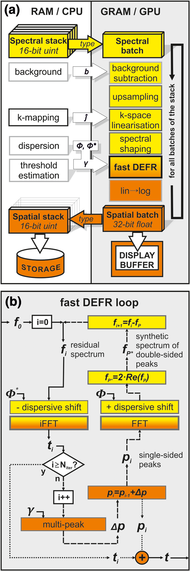

Since most OCT systems adopt C/C++ or LabVIEW as a coding tool for data acquisition and system control, while algorithm development is frequently performed in MATLAB, we demonstrate a strategy that employs a shared library compiled from MATLAB scripts to compute the FD-OCT processing in a practical OCT system. The MATLAB scripts were first compiled using the deployment tool to build a dynamic link library (DLL). Then programs written using VC++ (Visual Studio 2008, Professional Edition) invoked functions in this DLL to implement the DEFR algorithm on the GPU. The data communication between VC++ and MATLAB DLL was carried out by using mwArray Class in VC++.²³ The VC++ scripts were further compiled to generate another DLL which was available for other program platforms such as LabVIEW. In this project, we use LabVIEW (Version 2011, National Instrument, TX, USA) to implement GPU-based DEFR algorithm by calling a Jacket-MATLAB DLL via a C++ DLL.

3.

Results

Figure 2 shows a transverse scan in the horizontal meridian of an eight-week-old albino (MF1) mouse’s right eye, obtained by a 1060 nm SS-OCT system with $\sim 70\mathrm{nm}$ bandwidth, and the associated video demonstrates the graphic user interface during processing of the mouse-eye images. Details of the OCT system have been presented previously.²⁴ Figure 2(a) and 2(b) was calculated with the host CPU with double precision, while 2(c) and 2(d) utilized the GPU with single precision. Because the optical axis of mouse eyes is too long to be imaged with the “single-sided” depth range of the regular FD-OCT, we located the zero delay position inside the eye lens (denoted by a dashed line in the figure). It was found that the non-linear index vector calculated from a single calibration measurement in a free-space Michelson interferometer was sufficient for the $k$-space linearization of the raw spectra, thanks to the high sweep stability of the laser and no continuous recalibration was necessary. Figure 2(a) and 2(c) demonstrates the images directly reconstructed from dispersion-compensated spectra using a simple iFFT. Although the entire length of the eye is visualized, the images are compromised by the presence of “double-dispersed” conjugate components (indicated by arrows). From these images, it is difficult to measure the thickness of the crystalline lens, because the posterior lens surface is covered by the conjugate artifact of the cornea. Figure 2(b) and 2(d) shows the images generated by fast DEFR with 10 iterations and a stability parameter¹⁶ $\delta =0.5$. Complex conjugate artifacts were suppressed significantly without reducing sensitivity and axial resolution. In these figures the suppression of conjugate artifacts extends over the entire $z$-axis (depth) range, providing clear views of the cornea, lens, and retina. By comparison, there is nearly no qualitative difference between the corresponding CPU- and GPU-processed images, even when calculated at different computational precision. Figure 2(e) shows the differential image between Fig. 2(b) and 2(d), which is normalized to the system background-signal level. Numerical comparison verifies that the average remaining error in the worst case (single-precision GPU versus double-precision CPU) is $-8.2\mathrm{dB}$.

Fig. 2

In vivo transverse section in the horizontal meridian through the right eye of an albino (MF1) mouse. Image size: $4.21\times 8.11\mathrm{mm}$ ($512\times 800\text{pixels}$). Images were computed by (a) CPU without DEFR (b) CPU with DEFR, (c) GPU without DEFR, and (d) GPU with DEFR. (e) Normalized differential images between Fig. 2(b) and 2(d). The dashed line and arrows in (a) denote the zero delay position and the complex conjugate artifacts. Computation was implemented on CPU with double precision, on GPU with single precision. The grayscale values are normalized to the background-noise level. See also movie captured from the graphic user interface in processing the mouse eye images. (MOV, 3.27 MB) [URL: http://dx.doi.org/10.1117/1.JBO .17.7.XXXXXX.1].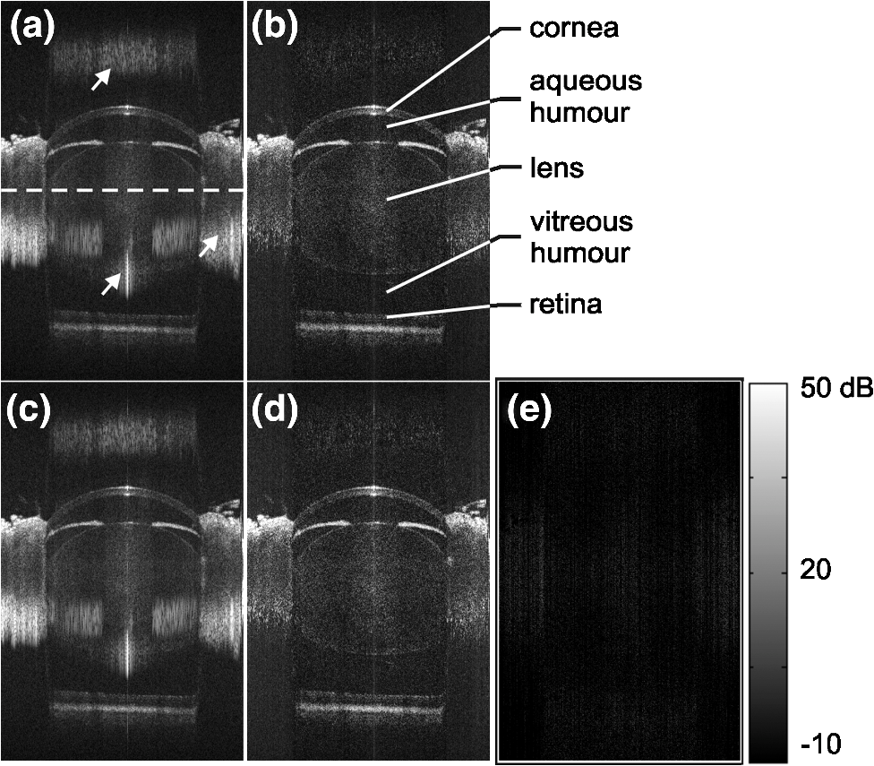

Codes were programmed in vector and matrix algebra as far as possible in order to maximize efficiency on the Jacket-MATLAB platform. For computation of a data batch, no cycle operations were employed except for the iteration in DEFR. Table 1 lists the average processing times with single precision and the speedup factors of GPU over CPU for a spectral batch of $512\times 2048$ samples in terms of the number of iterations. $N_{\mathrm{iter}}=0$ denotes that the images are directly reconstructed from dispersion-compensated spectra via iFFT. The samples in depth were doubled to 4096 in DEFR as we used an up-sampling factor of two. Since DEFR uses the dispersion mismatch, the computational time for digital dispersion compensation is included there.

Table 1

Processing times for a spectral batch of 512×2048 samples (mean of 100 tests, given in seconds) and speedup of GPU over CPU computing at single precision.

From Table 1, one can see the significant speed improvement of GPU over CPU. In the computation at single precision, speedup factors of more than $\times 90$ were achieved for the fast DEFR with GPU. The total time for 10 and 20 iterations was decreased to 43.92 and 69.61 ms from 3.28 and 6.07 s, resulting in speedup factors of $\times 74.78$ and $\times 87.20$, respectively. The former corresponds to a frame rate of $\sim 22.8\mathrm{f}/\mathrm{s}$ for high-resolution images, which is very close to video rate ($25\mathrm{f}/\mathrm{s}$). Expectedly, the runtime of DEFR is proportional to the number of iterations, while the sum of other processing time $T_{\text{other}}$ remains constant for both GPU and CPU. The speedup factor of DEFR is higher than that of $T_{\text{other}}$. Therefore, the overall speedup factor increases with the number of iterations.

Figure 3 illustrates the percentage of the GPU processing time for the case of 10 DEFR iterations in Table 1. DEFR and $k$-space linearization occupy 67% and 16% of the total GPU computational resource, respectively. Here, the time for the $k$-space linearization includes that for the up-sampling processing. The data transfer between the host and GPU memories takes a relatively small portion (9.39%) of the total computational time, which favors faster GPUs with larger numbers of processing pipelines.

Fig. 3

Percentage (mean of 100 tests) of the GPU time for processing a spectral batch of $512\times 2048$ sampling points with an up-sampling factor of two and 10 DEFR iterations. mem-cpy: data transfer between host and GPU memory.

Figure 4 shows the processing line rates of the GPU-based DEFR against the number of depth scans per batch. Each depth scan contains 2048 samples without up-sampling and the number of DEFR iterations is 10. The abbreviations used are Comp: the line rate for pure processing excluding data transfer and image display; Tot: the line rate including data transfer from host to GPU memory and back; and Disp: the line rate including image display, but excluding data transfer back to the host. For visualization, we used the Jacket image display codes to avoid GPU-CPU-GPU memory transfers. However, this might still involve GPU-internal data transfers. To provide a fair comparison, we cleared the GPU memory before testing the processing time when the batch size was altered. Figure 4 illustrates that initially, the line rates increase with batch size and reach a maximum of $\sim \mathrm{21,000}\mathrm{k}\text{-lines}/\mathrm{s}$ at $\sim 3,584$ depth scans per batch with synchronous display (Disp). Then, the line rates dramatically drop off above 4096 depth scans. In the experiment, we noticed that the peak memory access of the DEFR algorithm was proportional to the batch size with an increment rate of $\sim 152\mathrm{MB}/1024\mathrm{k}\text{-lines}$. The maximum graphic card memory usage was $\sim 1.0\mathrm{GB}$ for a batch size of 4096 depth scans, and out-of-memory errors occurred above 6656 depth scans.

Fig. 4

Processing line rates against depth-scan batch sizes. Each depth scan contains 2048 samples and the number of DEFR iterations is 10. Comp: computational time only; Tot: computational time + data transfer from host to GPU memory and back; Disp: Tot—data transfer back to host + image display.

In the LabVIEW implementation the program contained two concurrent threads, one for data (interference spectra) acquisition from external devices, and the other for signal processing. The program automatically assigned CPU cores to the threads, and the data were shared via global variables. The average processing time for a frame ($512\times 2048\text{samples}$, 10 DEFR iterations, up-sampling factor of two) was measured to be $\sim 68\mathrm{ms}$, corresponding to $7.5\mathrm{k}\mathrm{k}\text{-lines}/\mathrm{s}$. This speed was lower than that in Table 1 for the program on the MATLAB platform ($\sim 44\mathrm{ms}$), which may be attributed to multiple internal copies caused by LabVIEW when calling the DLLs.

4.

Discussion

In performance studies of GPU computing for standard FD-OCT by other researchers, the memory copy occupied $\sim 60\%$ of the computational resource.²⁰ Due to the relatively low computational-load-to-data ratio during FD-OCT, standard processing computation is memory-bandwidth limited. In contrast, DEFR is computationally about 10 times more expensive, thus the iterative reconstruction process dominates the post-processing time in DEFR OCT, while data transfer (9.39%, Fig. 3) is easily outweighed. However, the amount of data transfer in DEFR OCT and the processing in respect to signal content is only half the regular one, resulting in reduced data-transfer time/voxel. Because overall processing speed in upcoming GPU generations tends to progress faster than memory bandwidth, the algorithms will profit from newer GPUs as they are also positively affected by further process optimizations, such as compiled code and improvements in the programming environment.

Common computing tasks on CPUs are performed at double precision due to availability of optimized computing pipelines. In the field of GPUs, floating-point arithmetic was only recently supported. Especially in the cheap “consumer-grade” class of devices, double-precision computations are commonly not implemented or deactivated by the manufacturer and cost/performance calculations for the gaming industry result in large arrays of single-precision processing units on such devices. However, consumer demand has also raised support levels for double-precision GPU computing, although GPU manufacturers usually fully support high-performance computing only with costly speciality solutions. Despite different implementations double precision is more complex and generally slower. In view of the cost/performance ratio we investigated the physical and computational performance of GPU and CPU for DEFR with different floating-point types. Table 2 presents the ratios of processing times with double precision to single precision in Table 1. Both GPU and CPU are slower at double precision over single precision as expected. Interestingly, the ratio of cost to time for GPU is higher than that for CPU with double precision, resulting in lower performance gains. DEFR GPU and DEFR CPU need about 2× and 1.1× longer for double precision over single precision, respectively. For direct iFFT, the ratios are $2.6\times$ for GPU and $1.3\times$ for CPU. In order to investigate the effect of floating-point type on the image quality, we extracted the interference spectrum of a depth-scan in Fig. 2 for DEFR reconstruction with different floating-point types. Figure 5 plots the intensity profiles of an A-scan in Fig. 2 computed with single and double precision for different iterations. One can see that the results achieved at different computational precision increasingly differ with the number of iterations, but these alterations mainly remain within the noise background region affecting the signal-to-noise ratio (SNR) only at an insignificant amount. This is because the error caused by the computational inaccuracy accumulates throughout the iterations, until weak signals loose their coherence and further become part of the directionally ambiguous background. The images in Fig. 2 demonstrate that computation with single precision does not cause appreciable image-quality degeneration. We investigated the effect of precision on the SNR by simulating a signal at 1.0 mm depth position at $-42\mathrm{dB}$ SNR, and found the SNR loss was less than 0.2 dB in DEFR with up to 20 iterations. Therefore, it can be concluded that the floating-point type of single precision provides sufficient accuracy in DEFR OCT in practical situations. Both GPU and CPU can obtain computational acceleration with single precision, but the GPU implementation benefits more. In this context it has to be noted that the fast-DEFR algorithm with a lower number of necessary iterations profits from less numeric noise, which also means that an optimum setting of the amount of dispersion¹⁶ is of critical importance. Furthermore a lower density of scatterers, or the signal sparseness, is also beneficial for the algorithm and its residual (non-complex) background-elimination capability.

Table 2

Ratios of processing times at double precision versus single precision in Table 1, and ratio of GPU versus CPU processing at double precision.

Fig. 5

Intensity profiles of an A-scan in Fig. 2 computed with single and double precision. $N_{\mathrm{iter}}$: number of iterations. $N_{\mathrm{iter}}=0$ denotes that the images were directly reconstructed from dispersion-compensated spectra with iFFT.

As documented above, the processing speed of GPU-based DEFR relates to the batch size. It has been confirmed that the position of this inflection point around 4k samples coincides with the GPU memory size. DEFR OCT is a more complex algorithm than regular FD-OCT processing; therefore it requires more memory space for intermediate variables ($\sim 10\times$ in the current implementation). GPU cards with more memory can further contribute to an increased available batch size. However, it is still advantageous to optimize the codes further toward reduced memory requirements, although a batch size of 4096 is sufficient for most applications. To achieve the same depth range as in the half-range implementation (standard FD processing) only half the sampling points are needed for DEFR, which might be interesting in cases where sampling speed is the limiting factor. Due to the $n·\log (n)$ proportionality of the Fourier transform’s computational complexity with the sample number $n$, DEFR can also be speeded up by a factor of four. Furthermore, for less detailed previews, image quality can be sacrificed by avoiding up-sampling, which reduces computing time and increases the possible batch size. With the rapid development of consumer-grade GPUs from multiple competitors and continuous development of code optimizers, the processing line rate and the batch size of DEFR has the potential to scale to a couple of hundred k-lines/s and longer sampling depths. Recently released GPU architectures and GPU clusters already make the current DEFR code applicable for more demanding real-time visualization tasks that require higher line rates and depth ranges in ultra-high-resolution OCT and micro-OCT.

As a high-level interpreted language, MATLAB has the disadvantage of lower efficiency in respect to hand-tuned code that sometimes can reach performance gains with hardware-optimized code in the range of $\times 1.5$ to $\times 3$, and the same is true for hand-coded CUDA routines on the GPU. However, MATLAB provides fast matrix computation for vector processing to overcome this deficiency, together with a just-in-time compiler for code optimization. Also, its FFT operator employs the fastest Fourier transform in the West (FFTW), which is a C subroutine library for computing the discrete Fourier transform. In our previous work,¹⁶ a DEFR implementation in LabVIEW achieved a computation time of $\sim 1.8\mathrm{s}$ for five iterations ($512\times 2048\text{samples}$) with a 2-GHz CPU. This is comparable with the MATLAB version and might be improved in other, better optimizable environments. For GPU DEFR, the processing of a single iFFT (with dispersion compensation) took 0.0722 s, corresponding to $272\text{depth}\text{scans}/\mathrm{s}$. Reference 20 reported that their NVIDIA GTX295 Card (240 cores) achieved $680\text{depth}\text{scans}/\mathrm{s}$ for a frame size of $8192\times 2048\text{samples}$. Jacket-MATLAB adopts a garbage collection algorithm for memory management. Compared to C++, which allows both manual memory management as well as automated garbage collection,²⁵ MATLAB often consumes more resources but optimizes the code via a just-in-time compiler during runtime unless the code is already written in vectorized form. This may cause overhead memory allocation for variables, although the fixed dimension of variables in our codes significantly reduces the need to reallocate memory. Consequently, the Jacket-MATLAB software typically performs worse than hand-coded and optimized compiled CUDA as does MATLAB in respect to hand-optimized and compiled C/C++. Since in either case the most computationally expensive tasks (FFT and interpolation) are realized in compiled library subroutines, the performance gains might be attributed to the overhead of interpretation in MATLAB, Jacket, and LabVIEW in the current implementation. Even though the DEFR algorithm has been significantly accelerated by GPUs, it is still not available to process every captured image online in state-of-the-art, hundreds-of-kilohertz FD-OCT systems that surpass video rates. With the imaging-speed increase of OCT, the demand for improved processing methods always exists. Fortunately, in most applications it is not necessary or even possible to see every frame during measurement in real time. Usually, video rate ($25\text{frames}/\mathrm{s}$) display at high resolution ($\ge 512\times 512\mathrm{px}$) is sufficient for interactive operation. Besides, DEFR will undoubtedly benefit further from the development of the GPU and automated code-generation technology in the future.

To our knowledge, researchers in all the previous publications directly employed the CUDA language to develop and debug the GPU-based FD-OCT processing algorithms in the C/C++ environment. The complex direct programming of GPUs is still challenging and laborious to many engineers when developing and optimizing complex-signal-processing algorithms such as DEFR, Doppler-based motion extraction, and other analysis algorithms. In this paper, we demonstrate that easily accessible, high-level programming environments like MATLAB and Jacket on current consumer hardware can provide a means of answering the needs for computing complex medical-imaging algorithms in real time.

5.

Conclusions

In this paper, we presented a computation strategy for dispersion encoded full-range OCT for real-time complex-conjugate artifact removal based on a consumer-grade GPU and evaluated Jacket, MATLAB, as well as VC++ and LabVIEW as flexible programming platforms for FD-OCT processing. With GPU processing, the processing speed of DEFR could be improved by a factor of more than $\times 90$ over CPU processing for a typical tomogram size of 512 depth scans with 2048 samples and an up-sampling factor of two. The maximum display line rate of $\sim 21\text{kilo depth scans}/\mathrm{s}$ for $2048\text{samples}/\text{depth}$ scan at 10 fast-DEFR iterations was successfully achieved, thereby enabling the application of DEFR in fields where real-time visualization is required, e.g., for adjustment purposes. Due to the reduced numbers of iterations, the fast-DEFR algorithm also could be employed with single precision without significant deterioration in image quality. Besides other applications, the achieved computational speed matches the speed of common hard-drive-based storage devices, therefore filling the gap within the standard processing queue and shifting the information-processing bottleneck back to the analytic abilities performed by the investigator. In conclusion, adoption of GPUs for DEFR OCT will broaden its range of potential applications.