Autocorrelation noise removal for optical coherence tomography by sparse filter design

Hon Luen Seck; Ying Zhang; Yeng Chai Soh

doi:10.1117/1.JBO.17.7.076029

27 July 2012 Autocorrelation noise removal for optical coherence tomography by sparse filter design

Hon Luen Seck, Ying Zhang, Yeng Chai Soh

Author Affiliations +

Journal of Biomedical Optics, Vol. 17, Issue 7, 076029 (July 2012). https://doi.org/10.1117/1.JBO.17.7.076029

Abstract

We present a reconstruction method to eliminate the autocorrelation noise (ACN) in optical coherence tomography (OCT). In this method, the optical fields scattered from the sample features are regarded as the response of a sparse finite impulse response (FIR) filter. Then the OCT reconstruction is formulated as one of identifying the parameters of a sparse FIR filter, which are obtained via an ℓ1 optimization with soft thresholding. The experimental results show that the proposed method can obtain OCT reconstruction results with effective attenuation of ACN.

1. Introduction

Optical coherence tomography (OCT)¹ is a subsurface imaging technique that has gained popularity in many applications.²^–⁴ Since it was invented, time-domain OCT (TD-OCT) and Fourier domain OCT (FD-OCT) methods have been developed, among which the FD-OCT method has been recognized as the superior method due to its better sensitivity and higher speed.⁵^,⁶ In the FD-OCT method, the spectral interferogram measurements are regarded as the Fourier transform of the depth profile. However, the mutual interference of the optical field scattered from all the sample features also contributes to a part of the spectral interferogram. This gives rise to autocorrelation noise (ACN) in the FD-OCT reconstruction results. As the resultant ACN overlaps with the actual subsurface features in OCT images, the presence of ACN adds ambiguities when interpreting the OCT image.⁷ This is especially so in the case of full range detection or a sample consisting of several strong scattering layers with separations such that the ACN appears at the same location as the features of the depth profile. Thus, ACN is a major concern to the OCT community.

In order to eliminate the ACN, several approaches have been proposed. The simplest approach is to move the reference mirror away from the sample surface in terms of optical path. This approach reduces the influence of ACN but does not eliminate it. The second approach is to remove the mutual interference by using two or more phase-shifted spectral interferograms.⁸^,⁹ This approach eliminates ACN but requires multiple data acquisition. Furthermore, additional phase-shifted errors would complicate the matter.¹⁰ The third approach⁶ is to avoid ACN by reconstructing the optical fields scattered from the sample subsurface features and the reference mirror. Since the optical fields and the depth profile are direct Fourier transform pairs, the depth profile is reconstructed by Fourier transform without ACN. To uniquely reconstruct the optical fields, however, the minimum phase condition is required. This limits the class of samples in practice. The forth kind of approache is based on the cepstrum signal processing.⁷ The cepstrum of the optical fields is reconstructed first, from which the depth profile is obtained by Fourier transform. This cepstrum approach is applicable for a limited class of samples, as the approach requires the non-overlap of the cepstrums.

In this paper, the removal of ACN is carried out by exploiting the sparsity of the depth profile. The optical fields scattered from the subsurface features are regarded as the responses of a sparse finite impulse response (FIR) filter. Then, the OCT problem of reconstructing the depth profile from the spectral interferogram is formulated into one of identifying the parameters of a sparse FIR filter subject to its known spectrum. This problem can be solved by $ℓ_{1}$ -norm optimization by virtue of the sparsity. The modeling of scattered optical fields by a sparse FIR filter helps to remove the ACN. This is because the OCT reconstruction is carried out on the basis of a precise expression of spectral interferogram in terms of the depth profile and the mutual interference has already been taken into account in the reconstruction. But the challenge is that, in order to identify the sparse parameters of the FIR filter, $ℓ_{1}$ -norm optimization should be done subject to a quadratic constraint that relates the spectral interferogram to the depth profile. To overcome the challenge, an iterative soft-thresholding algorithm of $ℓ_{1}$ -norm optimization is developed. The performance of the proposed reconstruction method is evaluated by experiments, and the results are benchmarked against those of the cepstrum method and the minimum phase method. It is shown that the proposed method suppresses the ACN effectively.

2. Principle

The principle of the proposed method is illustrated by using the FD-OCT setup as shown in Fig. 1. The setup uses a fiber-coupled, low-coherence light source. The light beam goes through the fiber circulator and collimator, and it is split into the reference beam and the sample beam by the beam splitter. The sample beam penetrates the sample along the axial direction and it is reflected by the subsurface features at different depths. The reference beam is reflected at the reference mirror. Eventually, the light reflected from all the sample features and the reference mirror are coupled back into the fiber by the collimator. The coupled beams are then transmitted into an optical spectrum analyzer (OSA) that is usually designed with a fiber-coupled input. At OSA, the sample and light beams interfere and the raw spectral interferogram in the lambda domain is obtained. The interferogram would be used for constructing a single depth profile of the sample. Finally, the OCT image of the sample is constructed by assembling all the A-scan depth profiles with the assistance of the motion stage used to scan the sample laterally over the axial beam. Without loss of generality, the following discussion only considers recovering a single A-scan depth profile of OCT.

Fig. 1

Fourier domain optical coherence tomography (FD-OCT) setup.

In Fig. 1, we set up a $z$ -coordinate with the origin set as the position given by the zero optical path difference relative to the reference mirror. The coordinate system is used to indicate the positions of the sample features relative to the reference mirror. Furthermore, we introduce the following denotations. $E (t)$ denotes the optical field of low coherence light with $t$ denoting time instant, $E_{r} (t)$ denotes the optical field reflected from the reference mirror, $E_{s} (t)$ the optical field from the sample, $G (λ)$ the output optical spectrum of the low-coherence light source with $λ$ denoting the light wavelength, $R_{r}$ the reflectivity of the reference mirror, and $a (z)$ the depth profile to reconstruct.

From the system theory point of view, we can model the optical field of the low-coherence light as the output of a filter with spectrum given by $G (λ)$ , that is, $E (t) = G_{1} (q^{- 1}) e (t)$ , where $G_{1} (q^{- 1})$ is the transfer function of the filter, $q$ denotes a unit-time delay operator ( i.e., $q^{- 1} E (t) = E (t - Δ t)$ ), and $e (t)$ is an identically independent random sequence with unit power spectrum. Hence, the spectrum of the filter is given by $G_{1} (e^{i \frac{2 π c}{λ} Δ t}) G_{1} (e^{- i \frac{2 π c}{λ} Δ t}) = G (λ)$ , where $c$ denotes the light speed.

Similarly, the scattered optical field from the sample can be modeled as the output of a system with its input as the low-coherence light. Specifically, $E_{s} (t) = A (q^{- 1}) G_{1} (q^{- 1}) e (t)$ . Assume that absorption is weak or negligible. If we discretize the depth profile $a (z)$ into $a (k Δ Z)$ where $k$ is an integer and $Δ Z$ is the axial sampling rate, the scattered optical field can be considered as the sum of the input white light reflected from the scatters at the positions given by $k Δ Z$ with the reflectance of $a (k Δ Z)$ . In this sense, the unit-time delay can be considered as $Δ t = Δ Z / c$ and the transfer function $A (q^{- 1})$ is given by $A (q^{- 1}) = \sum_{k = 1}^{\infty} a_{k} q^{- k}$ with $a_{k} = a (k Δ Z)$ .

Then, the spectral interferogram is related to the sample features by the following expression:

Eq. (1)

S (λ) = ε [{| E_{r} (t) + E_{s} (t) |}^{2}] = ε [{| R_{r} G_{1} (e^{j \frac{2 π}{λ} Δ Z}) e (t) + A (e^{j \frac{2 π}{λ} Δ Z}) G_{1} (e^{j \frac{2 π}{λ} Δ Z}) e (t) |}^{2}] = G (λ) {| R_{r} + A (e^{j \frac{2 π}{λ} Δ Z}) |}^{2},

where

ε

denotes the expectation operator and the spectrum is obtained by substituting

q = e^{j \frac{2 π}{λ} Δ Z}

into the transfer functions

G_{1} (q^{- 1})

and

A (q^{- 1})

. It is worth pointing out that Eq. (1) actually tallies with the traditional expression of spectral interferogram

S (λ)

in FD-OCT.¹¹ Expanding the equation, the ACN term refers to

G (λ) A (e^{j \frac{2 π}{λ} Δ Z}) A (e^{- j \frac{2 π}{λ} Δ Z})

, which represents the mutual interference of all the optical fields scattered by the features of the sample.¹² However, the traditional expression of

S (λ)

is in wavenumber domain in FD-OCT.¹³ Here we express the spectral interferogram in wavelength domain for the reason that the spectral measurements are usually obtained in terms of wavelength. This has the additional advantage of avoiding the interpolation operation commonly needed in FD-OCT.

With the above models, the task of OCT reconstruction can be formulated as one of identifying the parameters of filter $A (q^{- 1})$ based on the available spectral measurements given by $S (λ)$ . In order to eliminate the ACN, the parameter identification should be done subject to the precise expression of $S (λ)$ in Eq. (1). In practice, the subsurface features observed by OCT are of sparse scatters. In view of this sparsity, we can consider a FIR filter of $A (q^{- 1}) = \sum_{k = 1}^{M} a_{k} q^{- k}$ , where $M$ denotes the order of the filter.¹⁴ The FIR representation means that there is only a finite number of optical path differences between the scattered optical field from the sample and the optical field reflected from the reference mirror. We can vary the order of the filter to consider different sparsity of the subsurface features.

Assume the spectral measurements are recorded by an OSA at $N$ wavelengths denoted by $λ_{n}$ . The spectral measurements available at an OSA are thus expressed as

Eq. (2)

S (λ_{n}) = G (λ_{n}) {| R_{r} + A (λ_{n}) |}^{2}, for all 1 \leq n \leq N,

where

Eq. (3)

A (λ_{n}) = \sum_{k = 0}^{M} a_{k} e^{- j k Ω_{n}},

with

Ω_{n} = 4 π / λ_{n} Δ Z

.

By considering the sparsity, the OCT reconstruction of the depth profile can be solved by the following $ℓ_{1}$ -norm optimization subject to quadratic constraint:

Eq. (4)

\min_{a} {‖ a ‖}_{1} subject to S (λ_{n}) = G (λ_{n}) {| R_{r} + \sum_{k = 0}^{M} a_{k} e^{- j k Ω_{n}} |}^{2},

where a is a vector with its

k

th element

a_{k}

and its

ℓ_{1}

-norm is defined by

{‖ a ‖}_{1} = (\sum_{k = 1}^{N} | a_{k} |)

.

In practice, the spectral interferogram obtained in the experiment is always corrupted by noise. This leads us to consider and solve the proposed method in the following mixed $ℓ_{1} / ℓ_{2}$ -optimization:¹⁵

Eq. (5)

\min_{a} {‖ a ‖}_{1} subject to \sum_{n = 1}^{N} {[S (λ_{n}) - G (λ_{n}) {| R_{r} + \sum_{k = 0}^{M} a_{k} e^{- j k Ω_{n}} |}^{2}]}^{2} < ϵ,

where

ϵ > 0

denotes the noise level.

The Lagrangian formulation of the optimization problem of Eq. (5) can be formulated as follows:

Eq. (6)

\min_{a_{k}} \sum_{n} \sqrt{{[e_{n} (a_{k})]}^{2}} + μ \sum_{k = 1}^{N} | a_{k} |,

where

e_{n} (a_{k}) = S (λ_{n}) - G (λ_{n}) {| R_{r} + \sum_{k = 0}^{M} a_{k} e^{- j k Ω_{n}} |}^{2}

, and μ is a regularization parameter that is required to control how stringent the quadratic constraint is μ performs the same role as

ϵ

does in Eq. (5).

Equation (6) can be solved by an iterative soft thresholding method.¹⁶ For this method, each iteration performs three main procedures: synthesizing, updating, and thresholding. In the procedure of synthesizing, an estimated value of $a$ is substituted into $G (λ_{n}) {| R_{r} + \sum_{k = 0}^{M} a_{k} e^{- j k Ω_{n}} |}^{2}$ to obtain the synthesized spectral interferogram denoted by $S (λ_{n}, a^{(i)})$ at $i$ th iteration. This procedure is denoted by applying a synthesis operator $Φ$ on $a$ , that is,

Eq. (7)

S (λ, a^{(i)}) = Φ \circ a^{(i)},

where

S (λ, a^{(i)})

is a vector with entries given by

S (λ_{n}, a^{(i)}) = G (λ_{n}) {| R_{r} + \sum_{k = 0}^{M} a_{k}^{(i)} e^{- j k Ω_{n}} |}^{2}

. In the next procedure, the estimate of

a

is updated by applying an adjunct operator

Φ^{*}

on the innovation given by

S (λ_{n}) - S (λ_{n}, a^{(i)})

. The updated estimate is given by

Eq. (8)

a^{(i + 1)} = a^{(i)} + γ Φ^{*} \circ [S (λ) - S (λ, a^{(i)})],

where

S (λ)

denotes a vector with entries given by

S (λ_{n})

, and

γ

is the gain used to control the updating procedure.

In the last procedure, the elements of $a$ are thresholded by using a soft thresholding function, $S T (x, μ)$ , given by

Eq. (9)

S T (x, μ) = {\begin{cases} x + μ, & x < - μ \\ 0, & - μ < x < μ \\ x - μ, & μ < x \end{cases},

where

x

is the function to be soft thresholded and μ is the threshold level. The choice of μ is experimentally determined, but it can also be determined by various criteria like the Akaike information criterion¹⁷ or the Bayesian information criterion.¹⁸

It can be seen from the above schematic of soft thresholding method that the key challenge in this method is to construct the adjunct operator $Φ^{*}$ in the updating procedure. By taking advantage of the FIR representation introduced in this paper, we propose one realization of $Φ^{*}$ as follows:

Eq. (10)

Φ^{*} \circ x = \sum_{n = 1}^{N} x_{n} e^{- j \frac{2 π}{Δ κ} (n - 1) κ_{n}},

where

κ_{n} = \frac{2 π}{λ_{n}}

,

Δ κ = (\frac{2 π}{λ_{1}} - \frac{2 π}{λ_{N}})

, and

x_{n}

is the

n

th element of

x

.

To summarize, the proposed OCT reconstruction method characterized in Eq. (4) or Eq. (5) can be implemented by the Algorithm 1.

Algorithm 1

OCT reconstruction with ACN removal.

Initialization:

Set the initial value of

a^{(0)}

, (e.g.,

a_{k}^{(0)} = 0

),

γ

, μ, and the total number of iteration steps

L

;

Compute the spectral interferogram by

b = Φ \circ a^{(0)}

by using (7);

Iteration:

Synthesizing: to compute the synthesized spectral interferogram

S (λ, a^{(i)}) = Φ \circ a^{(i)}

as in Eq. (7);

Updating: to calculate the new estimate

a^{(i + 1)} = a^{(i)} + γ Φ^{*} \circ (S (λ) - S (λ, a^{(i)}))

as in Eq. (8);

Soft thresholding:

a_{k}^{(i + 1)} = S T (a_{k}^{(i + 1)}, μ)

;

Output:

Output the reconstructed depth profile

a^{(i + 1)}

, until

i + 1

is equal to

L

.

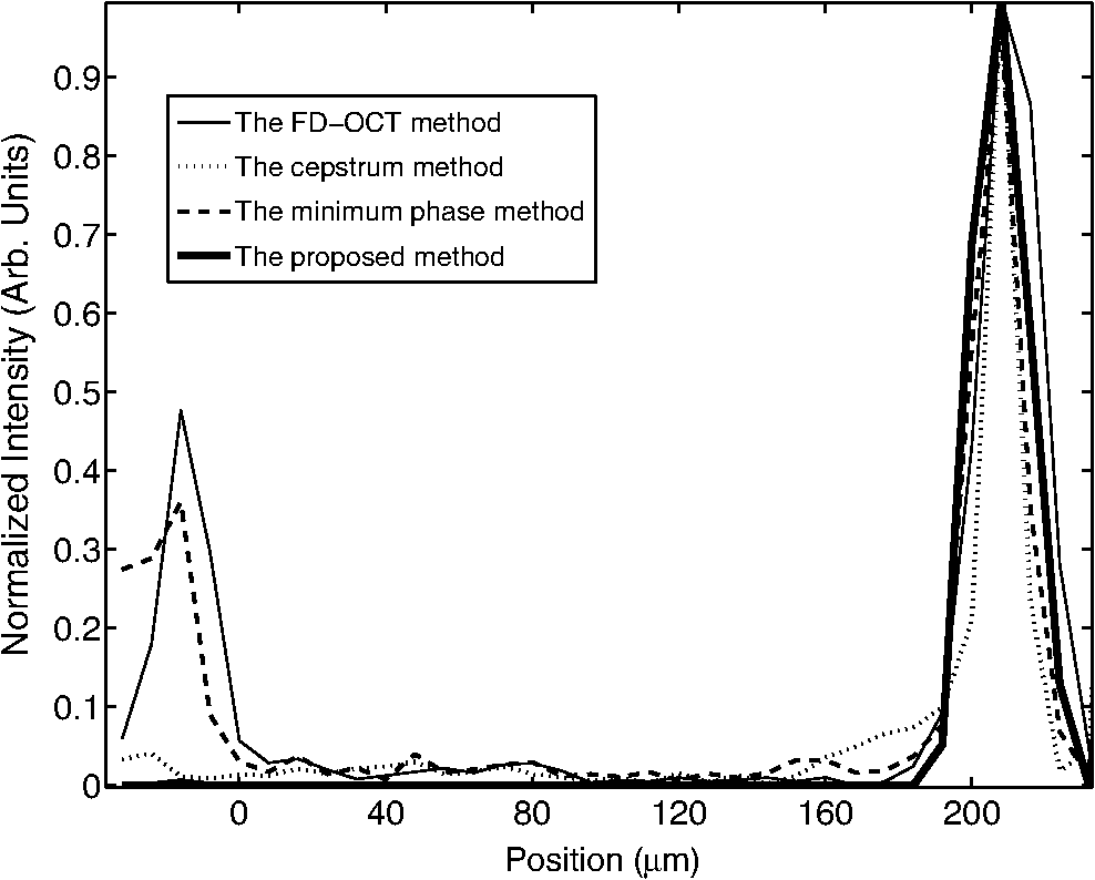
3. Performance of the Proposed Method

In this section, the performance of the proposed method is evaluated in terms of ACN removal capability, resolution, and computing demand. The performance is also compared to those of the FD-OCT method, the minimum phase method, and the cepstrum method. For a fair comparison, all the methods perform the reconstruction on the same set of the A-scan data, and the reconstruction is carried out on an Intel Core(TM)2 Quad CPU computer with 2.66 GHz processor and 4 GB RAM, and the software used is MATLAB 7.4 under 32 bits Microsoft Windows 7 operating system.

We begin with the evaluation of the effectiveness of the proposed method in removing the ACN. This is demonstrated and benchmarked by applying the method in two experiments to obtain OCT images. The first experiment uses a well-controlled sample formed by a two-mirror system. The second experiment applies the OCT method to image an onion sample. In all the experiments, the OCT is implemented on an interferometer setup as shown in Fig. 1. But for the second experiment, an additional microscope objective lens ( $Numerical aperature = 0.1$ ) is inserted between the collimator and the sample. This is to help collect the light reflected by the sample better. The light source used in experiments is a broadband Superluminescent diode (SLED 1550, Denselight) with the center wavelength at 1550 nm and the coherence length of 21 μm in air. The optical spectrum analyzer (ANDO6317B, ANDO) records the spectral interferogram with resolution 0.1 nm over a span of 154 nm centered at 1550 nm. It returns spectral measurements consisting of 1541 readings.

In the first experiment, a two-mirror system given in Fig. 2 is used as the sample in Fig. 1. The two mirrors labeled by $M 1$ and $M 2$ simulate the two interfaces of the sample. Mirror $M 1$ is carried by a motorized nanostage (Melles Griot 17NST101) and $M 2$ remains stationary. In this case, the depth profile consists of two spikes. Different depth profiles can be simulated by moving mirror $M 1$ . To carry out the experiment, the positions of mirrors $M 1$ , $M 2$ , and the reference mirrors are calibrated. The calibration of $M 1$ and $M 2$ is done with the reference mirror blocked and the OSA replaced with an optical power meter. The position of mirror $M 1$ is tuned until a maximum interference intensity is read at the optical power meter. The calibration of the reference mirror involves three steps. First is to block the mirror $M 1$ and unblock the reference mirror. Then, the position of the reference mirror is tuned until a maximum interference intensity is read at the optical power meter. Third, the position of the reference mirror is shifted until it is “in front” of both $M 1$ and $M 2$ by 120 μm. This gives the usual arrangement in OCT setup.¹³ After the calibration, all the mirrors are unblocked and the optical power meter is replaced with the OSA.

Fig. 2

Schematic of two-mirror system.

The OCT imaging is first performed to reconstruct an initial depth profile characterized by a position of mirror $M 1$ . Then, the OCT imaging is performed on different depth profiles simulated by moving mirror $M 1$ in steps. Finally, all the reconstructed depth profiles are assembled to give one OCT image. In each step, mirror $M 1$ is moved by 1 μm, and it is moved a total of 20 steps. At each step, the spectral resolution of the OSA is set to 0.1 nm, and a raw spectral interferogram is recorded over a span of 154 nm centered at wavelength 1550 nm. After the spectral interferogram is obtained, the depth profiles are reconstructed by different reconstruction methods including the proposed method, the Fourier transform–based FD-OCT method, the minimum phase method, and the cepstrum method. For the proposed method, the raw spectral interferogram is input into the Algorithm 1 with setting of $γ = 0.1$ , $μ = 0.001$ , $M = 300$ , and $L = 200$ . The reconstructed OCT image is shown in Fig. 3(d). For the remaining three methods, the raw spectral interferogram obtained at each mirror step is first spline interpolated to obtain a spectral interferogram that is uniformly sampled on wavenumber. For the Fourier transform–based FD-OCT method, each resampled interferogram is Fourier transformed using FFT, and all the depth profiles are assembled to give the depth profile image in Fig. 3(a). For the minimum phase method, the depth profile at each mirror step is reconstructed by using 1000 iterations of the algorithm proposed in the paper by Ozcan⁶ and the obtained depth profile image is displayed in Fig. 3(b). Figure 3(c) gives the corresponding result obtained by the cepstrum method.⁶

Fig. 3

ACN removal results: (a) FD-OCT method; (b) minimum phase method; (c) cepstrum method; (d) the proposed method. The arrows indicate the regions where artifacts are observed. (All the images are normalized and displayed in linear scale.)

For all the images in Fig. 3, the vertical axis denotes the dimension measurement over a range of 180 μm and the horizontal axis denotes the different positions of mirror $M 1$ . Comparing the images, the first observation is that the image obtained by the proposed method appears sharper than the others. Second, the ACN appears clearly in the top part of the image obtained by the Fourier transform–based FD-OCT method. They are suppressed in the image obtained by the minimum phase method and the cepstrum method, and they are totally eliminated in the image obtained by our proposed method. To see more closely, Fig. 4 shows a single depth profile obtained, respectively by the four methods. It is evident that an autocorrelation peak appears at $\sim 14$ μm position for the FD-OCT method, the minimum phase method, and the cepstrum method. But the ACN is eliminated by the proposed method. Summarizing the experimental results, it is confirmed that the proposed method can effectively eliminate the ACN. It is also noted that one of the feature peaks reconstructed by the proposed method is slightly lower than the one obtained by the FD-OCT method. This is attributed to the soft thresholding algorithm, which tends to underestimate the actual value.

Fig. 4

Depth profiles extracted from the images.

In the second experiment, the OCT imaging of a piece of onion skin is considered. Onion skin consists of hexagonal onion cell at the epithelium layer.¹⁹ The onion cell membrane forms the scatters which act as features in the depth profile. Thus, onion samples are often used to verify the OCT methods in the literature.²⁰ In this paper, the onion sample is prepared by placing a freshly sliced onion on the microscope glass slide having 1 mm thickness. Then, a thin layer of index-matching oil ( $r efractive index = 1.488$ ) is applied on the top surface of the onion skin, and another microscope glass slide with thickness of 100 μm is used to cover the onion sample. All glasses are made from BK7. Such a packaging is to remove the reflection from the bottom surface of covering glass slide, and the top surface of the covering glass slide can be used as a reference plane.

In the experiment, the packaged sample sitting on a nanostage (17NST101, Melles Griot) is placed under the microscope lens, and the position of the sample is adjusted vertically so that the top surface of the onion is at the focal plane of the microscope lens. The sample is scanned laterally over the microscope objective lens in steps of 1 μm over a range of 1 mm. At each lateral position, a set of A-scan spectral interferogram $S (λ)$ is measured over wavelengths with a span of 154 nm centered at 1550 nm. The measurements are obtained with the spectral resolution of OSA set at 0.1 nm.

After the A-scan spectral interferograms at all the lateral positions are obtained, we proceed to reconstruct the images by the proposed method, the FD-OCT method, the minimum phase method,⁶ and the cepstrum method,⁷ respectively. The reconstruction is done line by line, each line denoting one A-scan of depth profile. Then, the reconstructed cross-section OCT image resulting from the lateral scan is obtained by assembling all the A-scan depth profiles according to their lateral position. For each reconstruction method, the settings are the same for individual A-scans in the cross-section image. For the proposed method, the settings used in the Algorithm 1 are chosen as $γ = 0.4$ , $μ = 3.5 \times 1 0^{- 4}$ , $M = 500$ , and $L = 300$ . The cross-section image is shown in Fig. 5(a). For the other three methods, the spectral interferograms are first spline interpolated line by line to obtain another set of spectral interferograms, each of which is uniformly sampled on wavenumber. Then, Fourier transform is applied for the FD-OCT method, the algorithm described in the paper⁶ with 1000 iterations for the minimum phase method, and the procedure described in the paper⁷ is applied for the cepstrum method, respectively. The cross-section images reconstructed by the three methods are given, respectively in Fig. 5(b), 5(c), and 5(d).

Fig. 5

Onion imaging using various methods: (a) The proposed method; (b) FD-OCT method; (c) minimum phase method; (d) cepstrum method. The arrows indicate the regions where artifacts are observed. (All the images are raw images displayed without any image processing. They are normalized and displayed in logarithmic scale. Each image shows the cross section of the onion measuring 1 mm wide and 1.5 mm deep.)

Comparing the images in Fig. 5, it can be seen that there is a large area of artifacts on the top part of reconstructed image obtained from the Fourier transform–based FD-OCT. These artifacts are suppressed in the reconstructed cross-section images resulting from the proposed method, the minimum phase method, and the cepstrum method. However, since the artifacts are due to not only ACN but also other noises in practice, some left-over artifacts are still visible in the top parts of Fig. 5(a), 5(c), and 5(d). The second observation is the vertical artifacts appearing in Fig. 5(c) and 5(d). This may be due to two reasons. One is that the condition of non-overlap of the cepstrums is not satisfied for the depth profile at the corresponding positions. The second is the spurious artifacts as mentioned in the literature.⁷ But the vertical artifacts are totally removed in Fig. 5(a), which is obtained by our proposed method. Another observation when comparing the four methods is that the reconstructed image obtained by using our proposed method exhibits better clarity. This is because the method actually is based on an algebra reconstruction scheme which factored the point spread function in the reconstruction.

In the next part of this section, the resolution and computing demand of the various methods are compared. To evaluate the resolution, a quantitative measure called resolution gain (RG) is deployed here. This measure is commonly used in ultrasound imaging.²¹ It is calculated as follows. First, we calculate the autocorrelation function of one A-scan with respect to the depth position. Then, the autocorrelation function is normalized, with its maximum normalized to 1. The number of positions where the autocorrelation function is greater than 0.75 were counted to give the autocorrelation value. Second, we calculate the autocorrelation values, respectively on the A-scans of the proposed method, FD-OCT method, the minimum phase method, and the cepstrum method. Next, we use the one of the FD-OCT method as a reference, and calculate the ratio between this reference value and the autocorrelation values of other methods. This ratio is called the resolution gain. Without lost of generality, we consider the scenario of a mirror surface as the sample. The spectrum measurement is first simulated according to Eq. (1). Then, we apply respective method to reconstruct one A-scan, based on which we calculate the resolution gain for the method. The obtained resolution gains are summarized in Table 1. It is clear that the proposed method achieves the highest resolution gain. This implies that proposed method achieves highest resolution among various method. We attribute this to the inherent deconvolution properties of solving Eq. (5).

Table 1

Different performance measures.

Reconstruction method	Resolution gain	Computation time (seconds)	Autocorrelation noise removal capability
Proposed method	7	500	Best, due to algebra de-convolution helps to go beyond the coherence length
Minimum phase method	1.4	107	Good, but with spurious or vertical artifacts
Cepstrum method	1.4	6	Good, but with spurious or vertical artifacts
FD-OCT method	N.A.	4	None; the resolution is limited by the coherence length

The computing demand of various methods is evaluated by the computational time that is required by various methods to finish the reconstruction from one set of spectrum measurement. For each reconstruction method, we use the timer function in MATLAB to record the time needed. For the FD-OCT method, the minimum phase method, and the cepstrum method, the computational time also includes the time for spline interpolation of all the spectrum measurement and the time for FFT transform. The third column of Table 1 lists the computational time needed by the four methods to obtain the onion images in Fig. 5. It shows that the proposed method requires more time to perform the reconstruction. This is understandable, as the proposed method is based on an iterative reconstruction algorithm. This may mean that the proposed method achieves the high resolution at expense of computational time.

The overall performance of the proposed method and its comparison to other methods is summarized in Table 1.

4. Conclusions

A reconstruction method is proposed for the removal of the ACN in the reconstruction of depth profile by using OCT. The method is based on the modeling of the scattered optical fields in OCT by a sparse FIR filter. The depth profile reconstruction is formulated as one parameter identification problem of a sparse FIR filter given the spectrum response. The parameter identification is carried out via an $ℓ_{1}$ -norm optimization, but with a quadratic constraint. To overcome the challenge, an iterative soft thresholding scheme is developed in the $ℓ_{1}$ optimization to identify the filter parameters. Experiments and comparison studies show that the proposed method is able to remove the ACN from the OCT images effectively.

References

1.

D. Huanget al., “Optical coherence tomography,” Science, 254 (5035), 1178 –1181 (1991). http://dx.doi.org/10.1126/science.1957169 SCIEAS 0036-8075 Google Scholar

2.

O. P. BrunoJ. Chaubell, “Inverse scattering problem for optical coherence tomography,” Opt. Lett., 28 (21), 2049 –2051 (2003). http://dx.doi.org/10.1364/OL.28.002049 OPLEDP 0146-9592 Google Scholar

3.

P. E. Andersenet al., “Advanced modelling of optical coherence tomography systems,” Phys. Med. Biol., 49 (7), 1307 –1327 (2004). http://dx.doi.org/10.1088/0031-9155/49/7/017 PHMBA7 0031-9155 Google Scholar

4.

D. Stifter, “Beyond biomedicine: a review of alternative applications and developments for optical coherence tomography,” Appl. Phys. B, 88 (3), 337 –357 (2007). Google Scholar

5.

R. LeitgebC. K. HitzenbergerA. F. Fercher, “Performance of fourier domain vs. time domain optical coherence tomography,” Opt. Express, 11 (8), 889 –894 (2003). http://dx.doi.org/10.1364/OE.11.000889 OPEXFF 1094-4087 Google Scholar

6.

A. OzcanM. J. F. DigonnetG. S. Kino, “Minimum-phase-function-based processing in frequency-domain optical coherence tomography systems,” J. Opt. Soc. Am. A, 23 (7), 1669 –1677 (2006). http://dx.doi.org/10.1364/JOSAA.23.001669 JOAOD6 0740-3232 Google Scholar

7.

C. S. Seelamantulaet al., “Exact and efficient signal reconstruction in frequency-domain optical-coherence tomography,” J. Opt. Soc. Am. A, 25 (7), 1762 –1771 (2008). http://dx.doi.org/10.1364/JOSAA.25.001762 JOAOD6 0740-3232 Google Scholar

8.

M. Wojtkowskiet al., “Full range complex spectral optical coherence tomography technique in eye imaging,” Opt. Lett., 27 (16), 1415 –1417 (2002). http://dx.doi.org/10.1364/OL.27.001415 OPLEDP 0146-9592 Google Scholar

9.

A. F. Fercheret al., “Complex spectral interferometry OCT,” Proc. SPIE, 3564 173 –178 (1999). https://doi.org/http://link.aip.org/link/doi/10.1117/12.339152 PSISDG 0277-786X Google Scholar

10.

P. S. HuangS. Zhang, “Fast three-step phase-shifting algorithm,” Appl. Opt., 45 (21), 5086 –5091 (2006). http://dx.doi.org/10.1364/AO.45.005086 APOPAI 0003-6935 Google Scholar

11.

A. F. Fercheret al., “Optical coherence tomography—principles and applications,” Rep. Prog. Phys., 66 (2), 239 –303 (2003). http://dx.doi.org/10.1088/0034-4885/66/2/204 RPPHAG 0034-4885 Google Scholar

12.

V. M. Gelikonovet al., “Coherent noise compensation in spectral-domain optical coherence tomography,” Optic. Spectros., 106 (6), 895 –900 (2009). Google Scholar

13.

G. HäuslerM. W. Lindner, “Coherence radar and spectral radar—new tools for dermatological diagnosis,” J. Biomed. Opt., 3 (1), 21 –31 (1998). http://dx.doi.org/10.1117/1.429899 JBOPFO 1083-3668 Google Scholar

14.

F. J. Taylor, “,” Principles of Signals and Systems, Mcgraw Hill, Inc., New York (1994). Google Scholar

15.

M. ZibulevskyM. Elad, “L1-L2 optimization in signal and image processing,” IEEE Signal Process. Mag., 27 (3), 76 –88 (2010). ISPRE6 1053-5888 Google Scholar

16.

S. Mallet, “,” A Wavelet Tour of Signal Processing: The Sparse Way, Academic Press, Burlington, MA (2009). Google Scholar

17.

H. AkaikeB. N. PetroxF. Caski, in Proc. of 2nd International Symposium on Information Theory, 267 (1973). Google Scholar

18.

G. Schwarz, “Estimating the dimension of a model,” Ann. Statist., 6 (2), 461 –464 (1978). http://dx.doi.org/10.1214/aos/1176344136 ASTSC7 0090-5364 Google Scholar

19.

M. D. Kulkarniet al., “Image enhancement in optical coherence tomography using deconvolution,” Electron. Lett., 33 (16), 1365 –1367 (1997). http://dx.doi.org/10.1049/el:19970913 ELLEAK 0013-5194 Google Scholar

20.

H. L. SeckY. ZhangY. C. Soh, “Optical coherence tomography by using frequency measurements in wavelength domain,” Opt. Express, 19 (2), 1324 –1334 (2011). http://dx.doi.org/10.1364/OE.19.001324 OPEXFF 1094-4087 Google Scholar

21.

C. YuC. ZhangL. Xie, “An envelope signal based deconvolution algorithm for ultrasound imaging,” Signal Process., 92 (3), 793 –800 (2012). http://dx.doi.org/10.1016/j.sigpro.2011.09.024 SPRODR 0165-1684 Google Scholar

Citation Download Citation

Hon Luen Seck, Ying Zhang, and Yeng Chai Soh "Autocorrelation noise removal for optical coherence tomography by sparse filter design," Journal of Biomedical Optics 17(7), 076029 (27 July 2012). https://doi.org/10.1117/1.JBO.17.7.076029

Published: 27 July 2012

Access the abstract

JOURNAL ARTICLE
7 PAGES

DOWNLOAD PAPER SAVE TO MY LIBRARY

GET CITATION

CITATIONS

Cited by 5 scholarly publications.

Explore citations on Lens.org

RIGHTS & PERMISSIONS

Get copyright permission Get copyright permission on Copyright Marketplace

KEYWORDS

Optical coherence tomography

Mirrors

Optical filters

Reconstruction algorithms

Finite impulse response filters

Fourier transforms

Microscopes

1.

Introduction

2.

Principle

Fig. 1

Eq. (1)

Eq. (2)

Eq. (3)

Eq. (4)

Eq. (5)

Eq. (6)

Eq. (7)

Eq. (8)

Eq. (9)

Eq. (10)

Algorithm 1

3.

Performance of the Proposed Method

Fig. 2

Fig. 3

Fig. 4

Fig. 5

Table 1

4.

Conclusions

References

Show All Keywords

Keywords/Phrases

Search In:

Publication Years