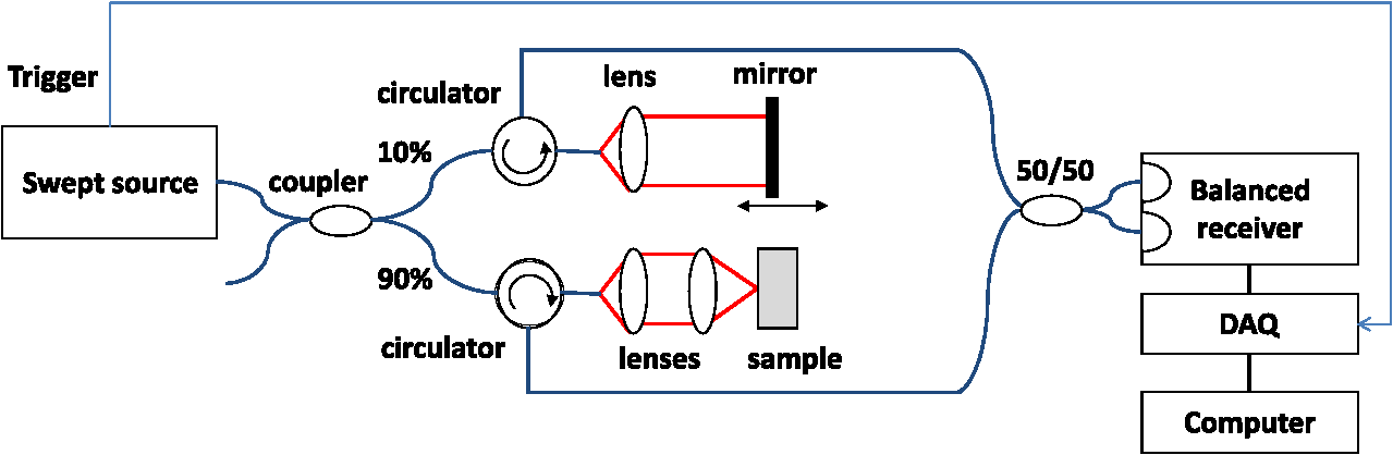
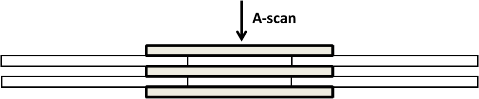
1.

Introduction

Optical coherence tomography (OCT) is an optical imaging technique that can provide non-invasive, cross-sectional, imaging of biological tissue with micrometer spatial resolution and intermediate (1–3 mm) depths.¹ With the introduction of fast, high-resolution, OCT systems, OCT technology has significantly improved over the past few years and is now well suited for in vivo applications. However, further improvements in resolution are required for the detection of many disease changes, such as those associated with early stage cancer, which are in the micrometer and sub-micrometer range. The axial resolution depends on the coherence length of the light source and is, thus, enhanced by the use of broadband sources. Kerr-lens mode-locked Ti:sapphire lasers, Ti:sapphire pumped super-continuum generation, and thermal light sources were used to obtain ultra-high axial resolution in biological tissue.^2–6 Additional extracavity spectral broadening in highly nonlinear fibers and simultaneous dual-band OCT with an off-the-shelf, all fiber, integrated supercontinuum source also provide ultra-high resolution.^7–9 In a recent paper, the generation of ultrabroadband biphotons that span a bandwidth of $\sim 300\mathrm{nm}$ with center wavelength ${\lambda }_0=812\mathrm{nm}$ has also been reported.¹⁰ Using these ultrabroadband biphotons in conjunction with semiconductor single-photon avalanche photodiodes (APDs), the narrowest axial resolution (0.85 μm) was reported in quantum OCT (QOCT). It was also shown theoretically that a chirped quasi-phase-matching nonlinear crystal structure can significantly enhance the axial resolution in QOCT by increasing the spectral width of the generated entangled photon pairs.¹¹ However, because the relationship between bandwidth and resolution is inversely proportional and asymptotic there is a limit to the resolution improvement that can be achieved even by these state-of-the-art OCT systems. Increasingly broader, often unattainable or unsustainable, bandwidths are required for marginal improvements in resolution. Also the system complexity and cost increase as the source bandwidth is extended and loss of sensitivity and power attenuation may ensue.

Numerical processing techniques have also been used to improve the resolution. An increase in resolution by a factor of $\sim 2$ can be achieved by the application of deconvolution techniques on OCT images as was first reported in 1997.¹² The CLEAN algorithm also yields promising results.¹³ Recently, two-dimensional deconvolution methods for deblurring were shown to improve the quality of OCT images as did the maximum entropy method (MEM) and Wiener-based autoregressive spectrum estimation (ASE).^14–16 In the latter case, a factor of 4 resolution improvement was achieved for time domain OCT (TDOCT) and a factor of 2 for Fourier domain OCT (FDOCT) images. All of the above techniques rely on processing and estimation from standard OCT data and do not take advantage of oversampling and modulation as does the technique proposed here. Moreover, by digitally reshaping the source spectra to known modes, OCT resolution improved by a few microns.¹⁷

In this work, a novel technique that effectively improves the axial resolution of Fourier domain OCT (FDOCT) without the need to use a light source with a broader bandwidth is demonstrated. The technique is based on the modulation and subsequent deconvolution of the interferometric OCT signal, a concept adapted to the Fourier domain but bearing some similarities to the method previously demonstrated in time domain OCT (TDOCT).¹⁸ The basis of this concept is the summation of more than one A-scans with different carrier frequencies and their subsequent deconvolution with appropriate kernels. This represents a method of achieving super-resolution by oversampling with both A-scans collected at the same sample location. However, the additional information which appears in the form of beating permits modulated deconvolution which significantly increases the resolution of the system. In FDOCT the real part of Fourier transform of each interferogram is modulated by a frequency which depends on the position of the interferogram in the $k$ space. If a signal is slightly shifted numerically, the frequency of the real part of the Fourier transforms changes. By adding two shifted interferograms, beating will appear in the A-scans. If the carrier frequencies are appropriately selected, the resulting interferogram will have a narrower width. Subsequent deconvolution, with suitable kernels, provides significant resolution improvement in FDOCT.

2.

Methodology

The method of resolution improvement proposed in this paper is based on two principles: (1) the appearance of beating after the addition of two waves of similar but slightly different carrier frequencies, and (2) the resolution improvement of the OCT images by deconvolution with a set of appropriately chosen kernel functions.

2.1.

Frequency Summation

In FDOCT the acquired signal from a single scatterer, e.g., a mirror, at position $r_0$ is:

Eq. (1)

$$S_{\mathrm{is}}(k)=[S(k)\cos (2\pi k{r}_0)]\otimes \delta (k-k_x),$$

where $S(k)$ is the spectrum of the laser source, $r_0$ is the location of the scatterer, and $k_x$ is the center location of the interferometric signal in the acquisition window which spans from $k_1$ to $k_N$. The real part of the Fourier transform of Eq. (1) is:

Eq. (2)

$$\text{Real}\{\mathcal{F}[S_{\mathrm{is}}(k)]\}=R_{\mathrm{is}}(r)=[R_{ii}(r)\otimes \delta (r-r_0)]\cos (2\pi k_{x}r),$$

where $R_{\mathrm{is}}$ is the cross-correlation of the source, and $R_{\mathrm{ii}}$ is the autocorrelation function. Equation (2) implies that the real part of the Fourier transform is modulated by a sinusoidal, whose frequency depends on the $k$ position of the interferometric signal, and the period of that sinusoidal is $1/k_x$.

If an interferogram is numerically shifted slightly, the period of the modulation changes. Adding two shifted interferograms can cause a beating pattern to appear if the amount of shift is appropriately selected. For example, consider

Eq. (3)

$${\mathrm{A}}_{i1}(\mathrm{r})=\text{Real}\{\mathcal{F}[S_{\mathrm{is}}(k)]\}=R_{\mathrm{is}}(r)=[R_{ii}(r)\otimes \delta (r-r_0)]\cos (2\pi k_{x1}r)$$

and

Eq. (4)

$${\mathrm{A}}_{i2}(\mathrm{r})=\text{Real}\{\mathcal{F}[S_{\mathrm{is}}(k)]\}=R_{\mathrm{is}}(r)=[R_{\mathrm{ii}}(r)\otimes \delta (r-r_0)]\cos (2\pi k_{x2}r)$$

that are two A-scans from shifted interferograms corresponding to the same single scatterer, where $i$ denotes the number of the A-scan in the image. The sum of the two A-scans is:

Eq. (5)

$$A_i(r)=A_{i1}(r)+A_{i2}(r)=[R_{\mathrm{ii}}(r)\otimes \delta (r-r_0)]\cos \left[\frac{2\pi r(k_{x1}+k_{x2})}{2}\right]\cos \left[\frac{2\pi r(k_{x1}-k_{x2})}{2}\right].$$

Filtering the carrier frequency $(k_{x1}+k_{x2})/2$ in Eq. (5), results in a demodulated A-scan with a beating frequency $(k_{x1}-k_{x2})/2$:

Eq. (6)

$$A_i(r)=[R_{\mathrm{ii}}(r)\otimes \delta (r-r_0)]\cos \left[\frac{2\pi (k_{x1}-k_{x2})r}{2}\right].$$

Figure 1 illustrates the basic principle behind modulated deconvolution. Figure 1(a) is the acquired backscattered signal from a sample consisting of 7 distinct reflections. Figure 1(b) is an interferogram from the same point but shifted in relation to the first. Characteristic beating patterns appear at each peak after summation of the two interferograms and Fourier transform. They are particularly evident when comparing a single peak from standard and modulated FDOCT in Fig. 1(d).

Fig. 1

(a) Backscattered signal from a sample consisted of 7 peaks, (b) signal from the same point shifted in relation to the first, (c) characteristic beating patterns at each peak after summation of two A-scans and FFT, and (d) a single peak from standard FDOCT and modulated FDOCT for comparison. Standard OCT is marked: red dashed line. Modulated OCT: blue solid line.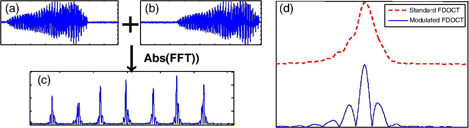

2.4.

Modulated Deconvolution, Resolution Enhancement, and Limitations

The axial resolution of an OCT image can be significantly improved, when modulated A-scans are deconvoluted with appropriate kernel functions.¹⁸ The equation of modulated deconvolution is derived from the TDOCT Eq. (25) in Ref. 18 and, for the case of an FDOCT A-scan, is:

Eq. (15)

$$R{s}_k\hat{h}(r)=h(r)=\sum _{k=1}^{N}h(r-r_k-\frac{\mathrm{\Delta }{\phi }_k-\mathrm{\Delta }{\phi }_m}{{\omega }_0}),$$

where $\mathrm{\Delta }{\phi }_{\kappa }=[{\phi }_1(r_{\kappa })-{\phi }_2(r_{\kappa })]/2$, $\mathrm{\Delta }{\phi }_m=[{\phi }_1(r_m)-{\phi }_2(r_m)]/2$, ${\omega }_0=2\pi \{[(k_{x1}-k_{x2})]/2\}$ and m is the number of the single peak used as kernel for deconvolution. The factor $(\mathrm{\Delta }{\phi }_k-\mathrm{\Delta }{\phi }_m)/{\omega }_0$ is the distance shift from the real position of each scatterer.

The simplest image deconvolution algorithm is the “inverse filter.” Because deconvolution in real space is equivalent to division in Fourier space, the inverse filtering algorithm divides the Fourier transform of an image by the Fourier transform of the point spread function (PSF). Although the calculation is rapid, the utility of this method is limited by noise amplification. During division in Fourier space, small noise variations are amplified by the division operation. The result is a trade-off between blur removal and noise gain. To avoid this trade-off a number of other algorithms have been developed for image restoration. These algorithms are the so-called “constrained iterative algorithms.” They work in successive cycles and also apply constraints on possible solutions. These constraints not only help to minimize noise or other distortions but also increase the power to restore a blurred signal.

One such algorithm is the Lucy-Richardson algorithm¹⁹ which is a technique widely used for restoring OCT images.^20,21 The reason for the popularity of this algorithm, which is based on a maximum likelihood implementation, is its ability to produce reconstructed images of good quality even in the presence of high noise levels.²² The algorithm maximizes the likelihood that the resulting image, when convolved with the PSF, is an instance of the blurred image assuming Poisson noise statistics. Because it uses probabilistic error criteria, this algorithm can provide slightly better restoration than other classical techniques. Also, since it takes into account statistical fluctuations in the signal and suppresses iterations when values deviate in the vicinity of their original value, it reduces noise amplification.²²

The Lucy-Richardson algorithm was used for the deconvolution operation in this paper. The Lucy-Richardson algorithm tends to concentrate energies near boundaries, which provides a good approximation to cellular boundaries and sub-cellular features, and tends to be more robust against errors from the defocused blur. Therefore, this algorithm offers the best performance for distinguishing physical features of the specimen at the cellular level.

2.4.1.

Axial resolution improvement with modulated deconvolution

By adding two interferograms, from the same sample location, shifted in $k$ space, beating will appear in the real part of the Fourier transform and the A-scan will have the appearance depicted in Fig. 1. As shown, there is already an improvement in the full width half maximum (FWHM) of the central lobe and, therefore, the resolution. The resolution improvement results from the fact that the modulated central lobe is narrower than the equivalent envelope of a standard OCT scan. The degree of the improvement depends on the modulation frequency and, therefore, the shift amount. The FWHM is the width $\zeta$ of the central lobe which can be calculated by combining

Eq. (16)

$$\sin \left[2\pi \right(\frac{k_{x1}-k_{x2}}{2})(r+\zeta )]=0.5\Rightarrow 2\pi (k_{x1}-k_{x2})(r+\zeta )=\frac{10\pi }{6}$$

Eq. (17)

$$\sin \left[2\pi \right(\frac{k_{x1}-k_{x2}}{2}\left)r\right]=0.5\Rightarrow 2\pi (k_{x1}-k_{x2})r=\frac{2\pi }{6},$$

which gives:

Eq. (18)

$$\zeta =\frac{2}{3(k_{x1}-k_{x2})}\mathrm{.}$$

Deconvolution contributes an additional resolution improvement of a factor of $\ge 2$ which results in:

Eq. (19)

$$\zeta =\frac{1}{3(k_{x1}-k_{x2})}=\frac{1}{3{\delta }_{k}n},$$

where ${\delta }_k$ is the sampling interval and $n$ is the shift in number of points. Equation (19) is equivalent to the TDOCT in Eq. (30) of Ref. 18.

The resolution improvement depends on the beating period since smaller beating periods result in narrower peak widths. Unfortunately the number and amplitude of the side lobes also increase at the same time.

2.4.2.

Side lobe amplitude and location shift

The appearance of side lobes is an important limitation of this technique. The relative amplitude of the first side lobe, which is the most severe case in terms of amplitude, is analytically calculated for TDOCT in Eq. (33) of Ref. 18. For the case of FDOCT signal, the side lobe amplitude is:

Eq. (20)

$$A_s=A_c{e}^{-{\left(\frac{\pi \mathrm{\Delta }k}{4(k_{x1}-k_{x2})\sqrt{\ln 2}}\right)}^2}=A_c{e}^{-{\left(\frac{\pi \mathrm{\Delta }k}{4{\delta }_{k}n\sqrt{\ln 2}}\right)}^2},$$

where $\mathrm{\Delta }k$ is the spectral width of the source, and $A_c$ is the peak amplitude. Equation (20) clearly illustrates that if the shift amount is larger and, therefore, the beating period is smaller, the amplitude of the first side lobe ($A_s$) is larger.

Another limitation of the technique is a location shift from peak to peak in the A-scan. As shown earlier, the real part of the Fourier transform can exhibit differences in phase between peaks. This leads to different beating patterns at different peak locations resulting in beating nodes at random locations relative to the center of the interferometric peak (Fig. 2). This introduces a shift in the location of the central lobe. The maximum location error can be derived from the TDOCT Eq. (37) in Ref. 18. For the case of FDOCT, the maximum error is:

Eq. (21)

$$\zeta =\frac{1}{2(k_{x1}-k_{x2})}=\frac{1}{2\delta k·n},$$

which implies that the maximum location shift is inversely proportional to the amount of shift between the two interferograms. The bigger the amount of shift the smaller is the distance error.

Fig. 2

Two different beating patterns resulting from two different scatterer locations of Fig. 1(c). (a) zero distance shift of the main lobe from the real position. (b), maximum distance shift of the main lobe from the real position. Intensity scales are linear. Standard OCT is marked: red dashed line. Modulated OCT: blue solid line.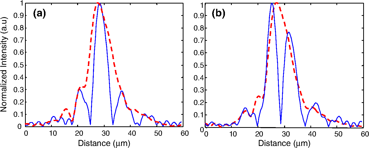

As explained above and illustrated in Fig. 2 the location shift and side lobe amplitude are a direct result of the different beating patterns at different locations. If the signal is deconvolved using as a kernel the beating pattern of Fig. 2(a), at locations similar to Fig. 2(b) there will be maximum distance shift and side lobe amplitude. However, if the beating pattern of Fig. 2(b) is used, the opposite will occur; i.e., the shift and side lobes will be worse at locations similar to Fig. 2(a). If both kernels are used, in successive deconvolutions, and the results are combined by multiplication, then the effect of distance shift and side lobe amplitude can be significantly reduced. It was noted experimentally that using three such kernels is adequate to minimize these issues. However, even after multiple deconvolutions, some uncertainty related to the initial phases of each interferogram remains.

2.4.3.

Design trade-offs

The tradeoff between side lobe intensity and number, location shift error, and resolution improvement is obvious from the above discussion. The greater the amount of shift between the interferograms, the smaller the distance shift error and the greater the resolution improvement. However, the number and intensity of side lobes also increases. A careful selection of shift is necessary to obtain optimal results for resolution improvement while maintaining the side lobe amplitude and location shift error within tolerated limits. From simulations and experimental data, it appears that an appropriate choice for the amount of shift is such that the beating pattern has a period of half the coherence length of the system. Such a value results in a resolution improvement of $\sim 7$ and a main side lobe amplitude 20 dB below the main peak after deconvolution. The side lobe amplitude is further reduced to 45 dB below the main with the use of three appropriate kernels. As with any design trade-offs, the values chosen will highly depend on system design and imaging study specifics.

3.

Experimental Method

Figure 3 shows the Swept Source OCT (SSOCT) system used in this study. The swept light source (Santec Corporation, Japan) had a 1310 nm-center wavelength, 110 nm FWHM bandwidth, and 20-kHz scan rate. 90% of the output power was coupled into the sample arm and the remaining 10% into the reference arm. Two circulators were used, in both the reference and sample arms, to redirect the back-reflected light to a $2\times 2$ fiber coupler ($50/50$ split ratio) for dual-balanced detection. The sample arm was scanned by tilting a mirror with a galvanometer. The dynamic range of the system (sometimes referred to as “sensitivity”) was 85 dB. This value was calculated as $10{\log }_{10}$ of the ratio of the square of the peak A-scan amplitude (generated by a perfectly reflecting mirror) to the variance of the noise floor (measured with the sample arm blocked). In the detection arm, the signal collected by the photodetectors was digitized using a 14-bit data acquisition board sampling at $40\mathrm{M}\mathrm{samples}/\sec$. The number of data points for each interferogram was 2000. The data acquisition start trigger for the digitizer was generated by the swept source. The depth encoded signal was calculated from the detected fringe signal by zero padding by a factor of four (increasing the number of points from 2000 to 8000), k-space resampling and Fast Fourier Transform (FFT). The sampling interval after zero padding and $k$ space interpolation was ${\delta }_{\kappa }=75.95$. The number of pixels we shift the interferogram is 3000. This value was chosen based on the trade-off discussion of Sec. 2.4.3 to provide the best possible results. These values also define the predicted resolution and error. The image range depth was 4 mm. The processing time is approximately 77 msec per A-scan pair on a 2.5 GHz PC using Matlab 2008.

Fig. 3

Configuration of the experimental swept source OCT system.

Images were acquired with continuous lateral scanning and oversampling in the lateral direction. Since adjacent A-scans were located at less than half the resolution apart, neighboring A-scans were considered to be identical. For every pair, one of them was appropriately shifted numerically. Beating appeared at each peak after adding the two and taking the real part of the FFT. In order to avoid filtering of the high frequency $(k_{x1}+k_{x2})/2$ in Eq. (13) we can take directly the absolute value of the FFT of the sum of two interferograms. This ensures a demodulated A-scan with beating at each peak with a beating frequency $(k_{x1}-k_{x2})/2$. A limitation of this experimental approach is that the acquisition time is twice that of standard OCT since two A-scans are acquired at each point in the sample.

A reference sample, consisting of three microscope cover slips of $\sim 170\mu \text{m}$ thickness spaced at $\sim 170\mu \text{m}$ distance (Fig. 4) was used to extract single peak interferograms subsequently used as kernels for the deconvolution. Of the resulting six peaks, three are chosen as kernels based on signal strength (i.e., the reflections with the strongest intensity are selected). Although it is not obvious that these kernels are the optimum for this procedure, they are adequate to provide acceptable results as explained in Sec. 2.4.2. This is a one time calibration scan which does not have to be repeated for every image.

Fig. 4

Sample consisting of 3 microscope cover slips ($\sim 170\mu \text{m}$ thickness, spaced at $\sim 170\mu \text{m}$ apart), used to collect the interferograms of 6 individual peaks from each A-scan.

4.

Results

The resolution of a system, as defined by Rayleigh, is its ability to discriminate adjacent structures in an image. In order to demonstrate the improvement in OCT resolution using the proposed method of modulation images were acquired from two glass microscope slides tightened together (Fig. 5). The two adjacent, inner, glass surfaces, with an air gap of $\sim 1.5\mu \text{m}$ between them (measured from the modulated OCT A-scans after processing) provided a suitable target for the evaluation of the system’s axial resolution. The kernels used for deconvolution are shown in Fig. 6(a) and 6(b). They were collected experimentally from the target described in Fig. 4. Figure 6(a) shows the kernels used for the deconvolution of a standard OCT image whereas Fig. 6(b) shows the kernels for the deconvolution of the modulated image.

Fig. 5

Sample consisting of two tightly adjacent microscope slides used to evaluate the resolving power of the proposed technique.

Fig. 6

Single peaks from (a) a standard OCT interferogram and (b) a modulated OCT interferogram used as kernels for deconvolution. (c) A-scan from standard OCT (dashed red line), and deconvolution of demodulated A-scans from standard (blue dash-dot line) and modulated OCT (black solid line) in one plot for comparison reasons. (d) Intermediate modulated deconvolution results for the first peak of (c). (e) and (g) Center peak of (c). (f) and (h) Last peak of (c). The $y$ axis is normalized to 1 for (a) and (b) and normalized to the highest peak of (c) for (e) and (f).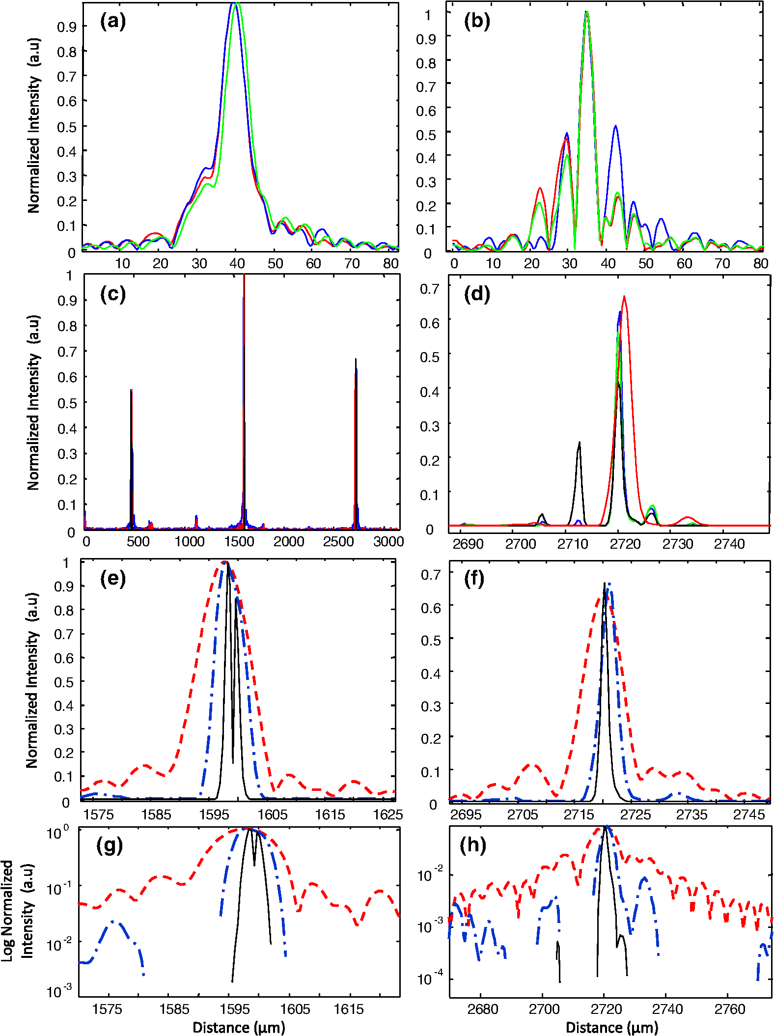

Figure 6(c)–6(h) illustrates the results of the proposed method and provide a quantitative measure of the resolution improvement achieved. Figure 6(c) is a plot of a single OCT A-scan showing the reflections from the faces of the two glass microscope slides. The middle peak is the reflection from the two adjacent middle surfaces, a close-up of which is shown in Fig. 6(e). The dashed red line is a standard OCT scan (with no deconvolution), the blue dash dot is the standard OCT scan after deconvolution with the kernels of Fig. 6(a), and the black line is the modulated OCT scan after deconvolution with the kernels of Fig. 6(b). The two adjacent surfaces were not discernible using standard OCT and appeared as a single peak. Even when deconvolution was performed on the standard OCT signal the two peaks were still not clearly resolved. With modulation and deconvolution the two peaks are unmistakably separated.

The improvement in the axial resolution of the system was quantified by examining the reflections from one of the single surfaces, in this case the peak at 2720 μm, a close up of which is shown in Fig. 6(f). The standard OCT resolution was measured to be 9.5 μm. After deconvolution of the standard OCT interferogram, the resolution improved to 4.2 μm and after applying modulated deconvolution was further improved to 1.4 μm, approximately a seven times improvement. This is consistent with the value predicted from the theory. The improvement is further verified by the clear separation (satisfying the Rayleigh criterion of resolution) of the two peaks in Fig. 6(e) which are at a distance of $\sim 1.5\mu \text{m}$ as estimated from that figure.

The technique was also tested on biological samples. Figure 7(a) shows a small region ($0.82\mathrm{mm}\times 0.96\mathrm{mm}$) of an onion image acquired with standard OCT. Figure 7(b) shows the same region after deconvolution of the standard OCT image. Axial resolution improvement is evident. Figure 7(c) is the onion image after modulated deconvolution. In this image, there is an improvement in resolution which results in the appearance of the characteristic onion double wall structures as evident from the zoomed regions of the same images in Fig. 8. The presence of the wall structure is also recognized in Fig. 8(d), which is a light microscopy image of onion cells. The distance between the cell membranes, measured from the modulated OCT images, was found to be between 6.8 and 8.2 μm, which is consistent with the literature (6 to 10 μm corresponding to the thickness of two cell walls). This is a case of new information, revealed using the proposed technique, which would have been previously unavailable.

Fig. 7

(a) Standard OCT image of an onion. (b) Same image after deconvolution. (c) Same data after modulated deconvolution. (Image size: $1.15\mathrm{mm}\times 1.35\mathrm{mm}$). The area in the red rectangle appears in Fig. 8. Intensity scales are normalized log.

Fig. 8

The area in the red rectangle of Fig. 7. (a) Standard OCT image of an onion. (b) Same image after deconvolution. (c) Same data after modulated deconvolution. (d) Light microscopy image of onion cells. (Image size: $0.65\mathrm{mm}\times 0.40\mathrm{mm}$). Intensity scales are normalized log.

Rabbit lung parenchyma was also imaged, ex vivo, to further demonstrate the applicability of the proposed technique to biological samples. The tissue was harvested immediately post termination and preserved in phosphate buffered saline at 4°C. Imaging was performed within about half an hour after harvesting. The zoomed images in Fig. 9(d)–9(f)) illustrates how the additional resolution improvement revealed small alveoli which in standard OCT appeared as highly back-reflecting dark areas.

Fig. 9

(a) Rabbit lung parenchyma imaged ex vivo with standard OCT. (b) Same image after deconvolution. (c) Same data after modulated deconvolution. (Image size: $1.2\mathrm{mm}\times 0.83\mathrm{mm}$). (d–f) Details of images (a)–(c), where small alveoli are indicated by the arrow. (g) Light microscopy image of a section of lung parenchyma from an unrelated site included for reference purposes. Intensity scales are normalized log.

In vivo images of skin were also processed with the proposed algorithm in order to demonstrate the applicability and effects of the technique on highly scattering biological tissues (Fig. 10). The fine tubular structure of the sweat duct is clearly visible after modulated deconvolution [Fig. 10(a), marked with d]. In addition, the effect of the methodology on speckle is also evident [Fig. 10(a), marked with s]. As expected from theory and prior work in time domain OCT,¹⁸ the speckle amplitude is not affected but its texture has become considerably finer.

Fig. 10

(a) In vivo, standard OCT, image of skin (finger tip). (b) Same image after deconvolution. (c) Same image after modulated deconvolution. (Image size: $1.15\mathrm{mm}\times 2.7\mathrm{mm}$). (d) Close up of the region marked with the rectangle in (a). (e) Same section after deconvolution of the standard OCT image. (f) Same image after modulated deconvolution. The area of the sweat duct (marked with d) clearly exhibits characteristic tubular structure. Areas of speckle are also indicated (marked with s). Intensity scales are normalized log.

To quantitatively assess the image quality in Fig. 7, the signal to noise ratio (SNR) and contrast to noise ratio (CNR) were calculated.

Table 1

Quantitative assessment of SNR and CNR of images in Fig. 7.

Applying Lucy-Richardson deconvolution improves the SNR of the image both in the case of regular deconvolution [Fig. 7(b)] and of modulated deconvolution [Fig. 7(c)]. This is a result of the property of the Lucy-Richardson algorithm to deblur the intensity of an image, therefore concentrating the power near the strong scatterering centers. This finding is consistent with literature.²¹ However, the CNR of the image decreases from 7.86 to 6.93 for the regular deconvolution and to 7.14 for the modulated deconvolution. In both cases, deconvolution decreases the CNR. However, the reduction is less severe for the case of the modulated deconvolution. These results are also consistent with the literature.²¹

5.

Conclusion

This paper demonstrates the application of modulated deconvolution in FDOCT to achieve superior resolution without the need of a broader bandwidth light source. The resolution improved significantly, in this case by a factor of $\sim 7$. Despite the limitations of this very preliminary implementation of modulated deconvolution, it is evident that this technique has the potential to dramatically enhance the resolution of OCT systems. In addition, different forms of encoding can be implemented in the future which will not suffer from the limitations uncovered in these experiments.