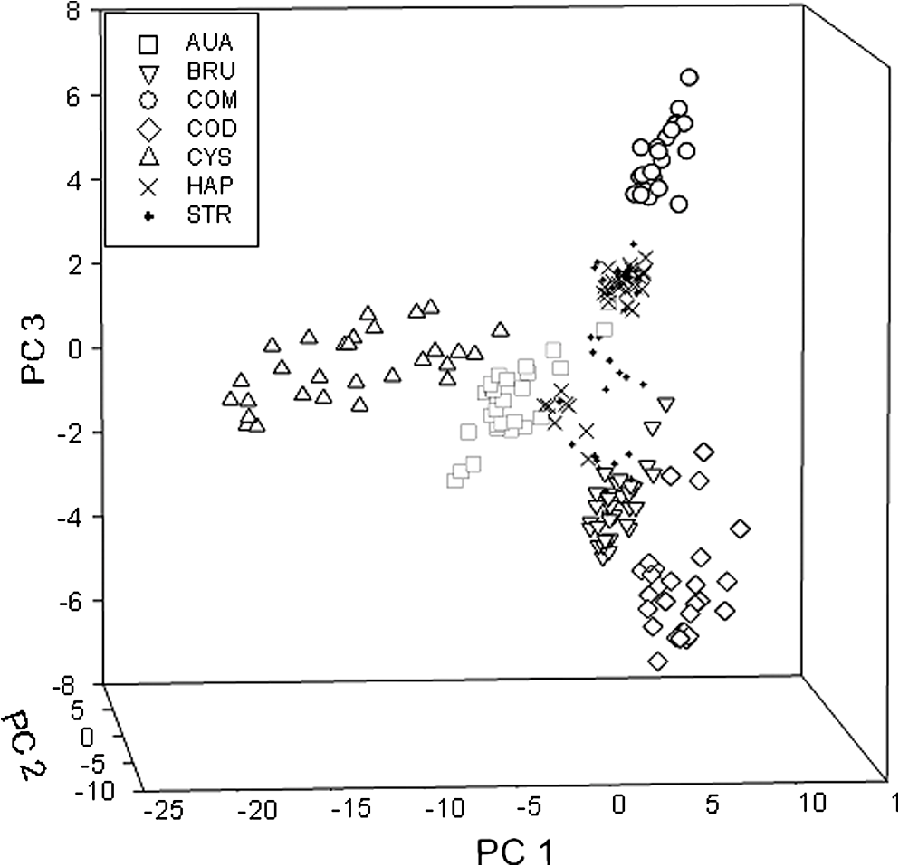
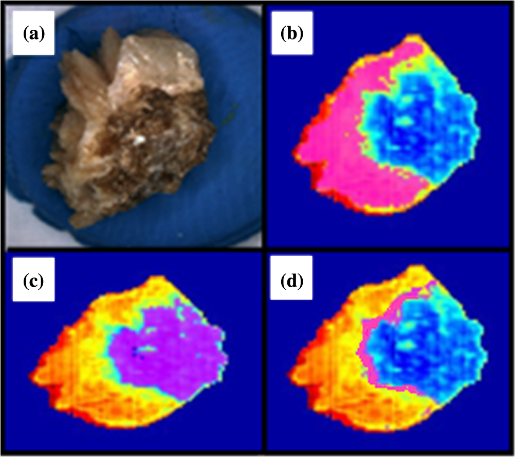
1.1.

Hyperspectral Imaging Technique

Hyperspectral imaging (HSI) or chemical imaging technique is based on the utilization of an integrated hardware and software architecture able to measure a spectrum for each pixel of the acquired image, being then possible to characterize the whole surface of the sample,^10,11 characteristics really useful for the objectives of the present work. It is desirable to analyze samples with flat surface because it always yields a better spectrum as the signal-to-noise (S/N) ratio increases due to better recording of the reflected radiation from the sample to the detector.

The acquired information is contained in a three-dimensional (3-D) dataset, characterized by two spatial dimensions and one spectral dimension, the so-called “hypercube”. According to the different wavelength and the spectral sensitivity of the device, several physical-chemical characteristics of a sample can be investigated and analyzed. For these reasons, HSI techniques represent an attractive solution for characterization, classification, and quality control of different products in many different fields, such as pharmaceuticals,^12,13 medicine,^14,15 food inspection,^16,17 artworks,¹⁸ and materials recycling.^19–22

There are two conventional ways to construct the hypercube; the first one known as the “staring imager” configuration and the second known as “pushbroom” acquisition.

The “staring imager” configuration keeps the image field of view fixed, obtaining images one wavelength after another.²³ Hypercubes obtained using this configuration thus consist of a three-dimensional stack of images (one image for each wavelength examined), stored in band sequential (BSQ) format. Wavelength in the “staring imager” configuration is typically moderated using a tuneable filter being the acousto-optic tuneable filters (AOTFs) or the liquid crystal tuneable filters (LCTFs), the most predominantly employed. AOTFs have been used in the construction of commercially available NIR-CI systems. The main advantages of AOTFs are the good transmission efficiency, fast scan times, and large spectral range. On the other hand, LCTFs show greater promise in filtering of Raman images due to the superior spectral bandpass and image quality.

The “pushbroom” configuration is based on the acquisition of simultaneous spectral measurements from a series of adjacent spatial positions, which require relative movement between the object and the detector.²⁴ Some devices produce hyperspectral images based on a point step and acquire mode: spectra are obtained at single points on a sample, then the sample is moved and another spectrum taken. Hypercubes obtained using this configuration are stored in the band interleaved by pixel (BIP) format. Advances in detector technology have reduced the time required to acquire hypercubes. Line mapping instruments record the spectrum of each pixel in a line of sample which is simultaneously recorded by an array detector; the resultant hypercube is stored in the band interleaved by line (BIL) format.

In this study, a “pushbroom” configuration was adopted, based on the utilization of a device of the ImSpector™ series spectrometers, developed by SpecIm™ (Finland). The spectrographs are constituted by optics based on volume type holographic transmission grating.¹⁰ The grating is used in patented prism-grating-prism construction (PGP element), characterized by a high diffraction efficiency, good spectral linearity, and nearly free geometrical aberrations due to the on-axis operation principle.

For handling of the huge amount of data available from HSI, chemometric techniques are required. Principal component analysis (PCA) is usually used for screening the raw data before the application of a classification technique such as artificial neural network (ANN). ANNs show an ever-increasing number of applications in many fields, since they can satisfactorily solve complex analytical problems.^25–27 Although simple in structure, the vast number of interconnections inside the ANN structure show an interesting potential for calculations.

The aim of the present study is to evaluate the application of HSI in the NIR field (1000 to 1700 nm) for the characterization and classification of renal calculi with the help of ANN, as this would be helpful for medical diagnosis, improving the conventional characterization done so far. In fact, HSI seems to be an interesting possibility to implement in hospital analyses where kidney stone samples have to be analyzed. This technique has already been used for testing a resolution method by analyzing two examples of kidney stones²⁸ and it has also been proved to be useful for other medical applications such as surgery monitoring.^29,30 However, HSI has not been deeply used for the study of kidney stones, once removed from the human body, or for the classification of the different types of kidney stones. On the other hand, ANNs have already been used in medicine with good results, even in urology,³¹ where the main applications have been related to cancer diagnostics and other illnesses, although they have never been used for the classification of kidney stones.

2.1.

Sample Preparation

Two hundred and fifteen samples were selected from a library of more than 1400 renal calculi. Samples were collected at the urology service of the Hospital, Universitari de Bellvitge, Barcelona (Spain). All kidney stones were obtained either by surgical removal or by natural expulsion. After collection, the stones were thoroughly rinsed with water and ethanol. Once cleaned, the stones were stored in individual clean vials showing no decomposition or damage in the structure during periods longer than a year.

Eleven types of different kidney stone components, including their mixtures, were considered. Firstly, seven main types of kidney stones were considered as formed by the pure compounds: uric acid anhydrous (AUA), brushite (BRU), calcium oxalate dihydrate (COD), calcium oxalate monohydrate (COM), cystine (CYS), hydroxyapatite (HAP), and struvite (STR). Secondly, mixtures of the former ones, namely: uric acid dihydrate (AUD), mixed calcium oxalate and hydroxyapatite (MXL), mixed calcium oxalate and hydroxyapatite (MXD), and COD transformed into COM (TRA) were analyzed. The selection criterion was based on variability appearance, for each type of stone.

For HSI technique, it is desirable to get a flat surface for the analysis, so all the samples were cut with a surgical knife, although it was also possible to measure and correctly classify round parts of stones. The inner part of the whole sample was used for the analysis, since the equipment allows the measurement of the entire stone. Besides, the use of the complete stone helped on the characterization of all its parts, contributing to the correct classification of each sample. Many samples showed a heterogeneous surface. In those cases, both the external part of the stone and the core were analyzed.

2.2.

Conventional Methodologies

Samples were firstly analyzed by means of stereoscopic microscopy. The analyses were carried out as described in the reported bibliography.^3,4 For those samples that were not well characterized by this method, an SEM-EDS analysis was performed.⁸ For this purpose, two different SEM equipments were used: JEOL JSM-6300 Scanning Electron Microscope (Japan), coupled to an Oxford Instruments Link ISIS-200 (UK) X-Ray Dispersive Energy Spectrometer (Univ. Autònoma de Barcelona); and a HITACHI S2500 (Japan) Scanning Electron Microscope, coupled to a Kevex 8000 (USA) X-Ray Dispersive Energy Spectrometer (Univ. “La Sapienza” of Rome). The structure of the samples was analyzed, and the EDS analysis was performed on some parts of the stone to confirm the elemental composition of the sample. Some representative results are shown in Figs. 1 and 2.

Fig. 1

SEM images of the internal part of some kidney stones. (a) AUD, (b) COD, (c) COM, and (d) HAP.

Fig. 2

Mapping experiments on the surface of a kidney stone. (a) SEM image of some a struvite kidney stone; (b) mapping for Mg; and (c) mapping for Ca.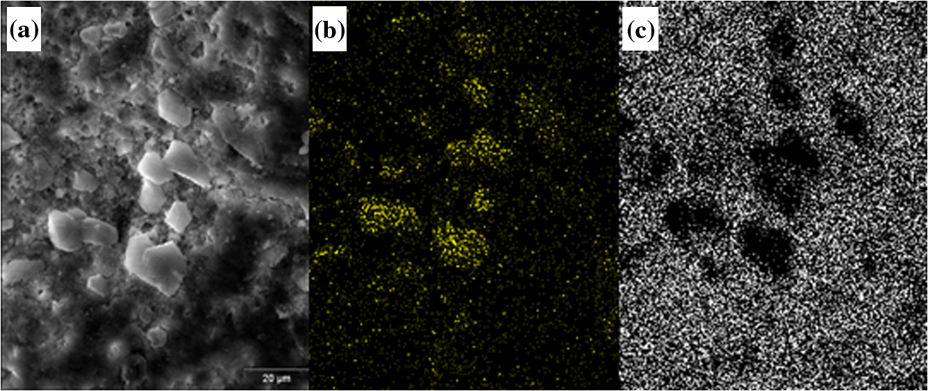

The results coming out from these conventional methodologies were used as references for the results obtained from HSI data.

2.3.

Hyperspectral Imaging Device and Architecture Set-Up

The HSI system used (Univ. “La Sapienza” of Rome) was constituted by the following components: optics, spectrograph, camera, translation unit, energizing source, and control unit (Fig. 3). The core of the system was a spectral camera NIR (Specim, Finland) embedding an ImSpector™ N17E imaging spectrograph working in the wavelength region 1000 to 1700 nm and a Te-cooled InGaAs photodiode array camera (spatial resolution: rms spot radius $<15\mathrm{\mu m}$; spectral resolution: 7 nm; 121 wavelengths measured).

Fig. 3

HSI based architecture employed for the acquisition of the kidney stones spectra.

The spectrometer was coupled to a 50 mm lens. The resolution of the image width was 320 pixels, while the number of frames, that is, the resolution of the image in the $Y$ axes varied from 200 to 350 pixels, depending on the number of samples measured at a time.

The energizing source was constituted by a diffused light cylinder with aluminium internal coating, embedding five halogen lamps that produce an intense and continuous spectrum signal, which was optimized for the NIR region.

The spectral camera was hosted in a laboratory platform equipped with an adjustable speed (from 0 to $50\mathrm{mm}/\mathrm{s}$) conveyor belt ($\text{width}=26\mathrm{cm}$ and $\text{length}=160\mathrm{cm}$). Spectra acquisition can be carried out continuously or at specific time intervals. The device was fully controlled by a PC unit equipped with the Spectral Scanner™ v.2.3 acquisition/preprocessing software (DV srl, Italy).

The spectra of the samples were measured fixing them to a plastic holder with the inner side upwards, so the core was visible to the detector.

The stones previously classified as pure compounds, by means of conventional methodologies, were used for creating a library of compounds, which could be later applied for the classification of unknown samples.

2.4.

Spectra Handling

The acquisition of the spectral signatures was carried out after a preliminary calibration performed in two steps: i) black image acquisition and ii) measurements of “white reference image” using a standard white ceramic tile. After the calibration phase, the spectral image was acquired and the reflectance ($R$) was computed according to the following equation:

The analysis of the stones was performed on five randomly selected region of interests (ROIs) on the surface of the sample in order to avoid the selection of any part of the stone that might contain organic matter. Then, all the regions in a sample were considered as a single sample for data treatment. Although the ROIs analysis loses the information for every single pixel, it has two main advantages. First, it is a way of smoothing the data, since the surface of the sample might not be homogeneous considering adjacent pixels due to organic matter which could have been trapped into the structure of the stone during the crystallization process. Second, the amount of information that is going to be handled is much smaller than in the analysis of the full pixel matrix.

Additionally, an image analysis for each individual pixel was performed using a PCA treatment to show the capabilities of this technique for handling entire images on the classification process.

2.5.

Data Treatment

For the analysis of the data, three different methods were used: factor analysis (FA), PCA, and ANN.

Although FA and PCA share the same main goal, that is, the reduction of the number of variables of the system by finding latent connections between real variables, they have a basic difference that allows obtaining different information.³²

FA is based on correlation between variables, and the number of factors considered descriptors of the system is selected according to the associated eigenvalue.^33,34 Several criteria have been suggested in order to decide this number of factors. Kaiser’s rule, which states that only those factors with an associated eigenvalue greater than 1 are representative for the system,³² has been applied in this study. All other factors stand for linear combinations of real variables, describing only noise.

On the other hand, PCA is based on the variance of the data.³⁵ Therefore, the main principal component (PC) for the system follows the direction in which the data have a bigger variance.

Due to these properties, FA was used to check how many different components can be distinguished in all the samples, while PCA was useful for the variable selection.

With regard to ANNs, they are considered a sophisticated and powerful computational tool which solves difficult analytical problems by learning from real cases. An ANN is a computational model formed from a certain number of single units, artificial neurones or nodes, connected with coefficients (weights), $w_{ij}$, which constitute the neural structure. Despite many different structures that ANNs can take, already described in the literature,^25,36 the structure used in this study was constituted by three layers: inputs, one hidden layer, and outputs. The input layer receives the information about the system (the nodes of this layer are simple distributive nodes, which do not alter the input value at all). The hidden layer processes the information initiated at the input, while the output layer is the observable response or behavior. The algorithm chosen for the learning process was the backpropagation. The optimization of the ANN was carried out by minimizing the root mean square (RMS) error,³⁷ when modifying the number of nodes in the hidden layer.

2.6.

Software

HSI data has been treated using the following software: STATISTICA (Tulsa, OK);³⁸ The Unscrambler v 9.1 (Camo Process, Oslo, Norway);³⁹ MATLAB v 7.0 (MA, USA),⁴⁰ PLS toolbox by Eigenvector Research, Inc. and TRAJAN v 3.0 (Horncastle, UK).⁴¹

3.1.

Factor Analysis

The software STATISTICA was used to perform FA on the data. The data used for this analysis was the spectra corresponding to the seven types of different components, since they represent the whole variety of substances studied.

Figure 4 shows how the weight of the Eigenvalue associated to each factor decreases for less important factors, being the seventh factor the last one having a value greater than 1. According to Kaiser’s rule, it can be seen that FA distinguishes the main species forming renal calculi.

Fig. 4

Eigenvalues for the seven main groups of renal calculi and explained variance for the PCA model. Model A: reflectance data, Model B: first derivative.

Taking into account these results, a PCA analysis was carried out in order to create a model that is able to classify the different types of kidney stones analyzed.

3.2.

Principal Components Analysis

PCA was used for screening the spectral data. It was useful for selecting variables before performing the classification, which was made using ANNs.

3.2.3.

Variable selection

Multivariate methods can certainly give a higher amount of information than univariate ones, though many variables from the measured range might not give valuable data, but noise. In this sense, we can take advantage profit from the fact that one of the basic statements of PCA is the reduction of number of variables, by taking only the information contained in the independent variables. Actually, not all the regions of the NIR spectrum give relevant information to the model. Then, by choosing those wavelengths with the greatest classification capabilities, the noise of the system is reduced thereby increasing its precision and simplifying the calculations.

To achieve this goal, the selection of variables is based on their loading value. In a PCA analysis, the loadings stand for the weight that every real variable has on each of the principal components. The wavelengths to be taken into further calculations are those that have a highest value for the loading for each PC. The representation of the loadings of every wavelength for each PC (Fig. 5) is a clear way to see the most important wavelengths, since it can be seen which regions of the spectrum are mostly influencing for a given PC. On the other hand, the regions of the spectrum that have a bigger weight on a given PC should correspond to the vibration wavelength of the compound classified by this PC.

Fig. 5

Loadings of each variable for the seven first PCs.

Following the above mentioned path, it was possible to define the variables defining every compound from the information in Fig. 5 and the representation of the scores values, see results in Table 1.

Table 1

Characteristic NIR vibrations for each type of renal calculi.

Type of kidney stone	Characteristic PC	$\mathrm{\Lambda }$ with highest loading (nm)	Associated NIR vibrations
CYS	$\mathrm{PC}1<0\cdots \mathrm{PC}2>0$	1188–1230, 1440–1542	CH, ${\mathrm{CH}}_2$, ${\mathrm{CH}}_3$
AUA	$\mathrm{PC}1<0\cdots \mathrm{PC}2<0$	971–978, 1083–1167	Ar-OH
COD	$\mathrm{PC}3>0\cdots \mathrm{PC}2>0$	1426–1475	${\mathrm{H}}_2\mathrm{O}$
COM	$\mathrm{PC}3<0\cdots \mathrm{PC}4>0$
BRU	$\mathrm{PC}3<0\cdots \mathrm{PC}4<0$	1223–1244	CH
HAP	Not well defined
STR

3.3.

ANN: Optimization of the Neural Network

The software ‘TRAJAN’ was used for creating the ANN model, using the first derivative of the reflectance spectra measured.

The raw data of the spectra contain all the measured wavelengths, so in order to decrease the number of variables in the system 50 wavelengths were selected according to the values of the loadings for each wavelength, as shown in Fig. 5. In this way, a matrix of 140 samples (seven main types of kidney stones) and 50 variables was used for the analysis.

The ANN to be optimized was defined as: (inputs, number of nodes in the hidden layer, outputs), where inputs stand for the number of samples used to create the model, and outputs, the number of types of kidney stones, that is (140, n, 7). The value for the outputs was a single variable, which could take up to seven different nominal values.

The algorithm used for the optimization of the structure was the backpropagation. After the optimization of the ANN, it was seen that the optimum number of nodes in the hidden layer was four, and the value after which a non decrease in the RMS error²⁴ was observed. To avoid an overfitting of the model, no more nodes were used.

4.1.

PCA and Variable Selection

It has been seen that PCA allows for the determination of the main variables that define the system. For instance, the scores and loadings for PC2 can be also analyzed (see Fig. 6). In this case, AUA and CYS have opposite scores sign, meaning that PC2 is clearly differentiating between these two components. PC2 is well defined with positive loading values for wavelengths from the ranges 1188 TO 1230 nm and 1440 to 1542 nm. All these vibrations are associated to C–H bond vibrations. This association perfectly fits with the structure of cystine, since this is the only component of the studied set which has C–H bonds. On the other hand, wavelengths 971 to 978 nm and 1083 to 1167 nm have negative loading values for PC2. In this case, the associated bond vibrations are the Ar-OH, which can be related only to AUA.

Fig. 6

3D representation of scores for PC1, PC2, and PC3.

Additionally to this case, some other data defining the rest of compounds can be observed in Table 1. Clearly, the vibration differentiating COM and COD is the band for water.

It can be appreciated that the NIR bands that define BRU appear in the range of C–H vibrations. This fact might be explained due to especially high amount of organic matter contained in BRU calculi, since no C–H bonds are found in brushite structure.

The main drawback the PCA has shown was the difficulty to distinguish HAP and STR results which can be clearly seen in Fig. 6, where these two compounds appear as two overlapped clusters. These results can be understood because of their very similar composition. Struvite calculi are basically hydroxyapatite stones with a variable amount of struvite crystals spread within the whole stone. It means that most of the sample is similar to a pure HAP kidney stone.

Though the only exception of HAP and STR renal calculi, the PCA analysis has shown to be useful for the classification of the components of kidney stones.

4.2.

Image Analysis

A different PCA analysis was also performed on the seven groups of kidney stones, taking directly the hyperspectral cube and using the software MATLAB.

One sample from each type of kidney stone was analyzed, getting a classification pixel-by-pixel. As in the previous PCA, the data used was the first derivative of the spectra and the data were again mean centered.

Some samples considered pure compounds (as characterized by means of stereoscopic and SEM-EDS microscopies) were used to create a model for later classification of unknown samples.

The identification of the different compounds was done by interpretation of the colors obtained when creating reconstructed RGB images from the hyperspectral cube. When using this kind of representation, the scores values for each of the 3 PCs used for the plot will determine the color of the pixel.

Figure 7 shows different colors for each kind of kidney stones, providing a simple way to distinguish a type among the others, except for STR and HAP. Indeed, the results obtained analyzing the hyperspectral cube completely matched with those obtained by taking ROIs from the samples.

Fig. 7

RGB image for the seven main groups of renal calculi.

Moreover, the software allows the selection of a group of pixels from the scores representation. Therefore, it is possible to identify which area of a sample or group of samples contain a given compound, when the scores values of each one are known.

An example is shown in Fig. 8. Three different areas are highlighted: COD, COM, and the interface, namely TRA. This last compound is the result of the slow change that the COD (kinetic derivative) undergoes into COM (more stable).

Fig. 8

(a) Image of the real stone; highlighted: (b) COD, (c) COM, and (d) TRA.

4.3.

ANN Performance

The model was applied to the seven groups of main compounds forming kidney stones, using the previous conditions. The results, checked with cross-validation leave-one-out, show up to 100% of accuracy for the classification.

The next step was to further reduce the number of variables in the system, so that the foretold advantages of the variable reduction become clearer. With only 30 wavelengths selected, the accuracy for the classification remained at 100%.

When even less variables are taken for the calculations, the percentage for right classification dropped down to 95% at most. Consequently, the final choice was the model including 30 wavelengths.

However, due to the importance of a precise classification regarding the diagnostic for the patient, the really interesting objective is the classification of 11 groups of different types of kidney stones, that is, the seven main compounds and their mixtures.

Thus, an optimization of a new ANN model, capable for the classification of this much more complex data was required. For this purpose, 50 wavelengths were introduced as variables, being the structure of the optimized ANN (215, 13, 11). In this case, the rate of well-classified samples reached 94.4%. The reader is referred to Table 2 for the accurate classification of the set of 215 samples of kidney stones used for this study showing the classification obtained by the conventional technique and that developed in the present work.

Table 2

Comparison between the results obtained using conventional techniques (stereoscopic microscopy and SEM) and the new developed methodology (HSI-ANN). Note: For the classification of the samples by HSI, a library of substances was defined with some stones considered as pure compounds. The items highlighted are the erroneously classified.

As seen in this Table, the error for the last model, including all types of kidney stones, is only slightly higher than that for the simpler model. Nevertheless, the second model offers a great advantage, since it is able to deal with any of the kidney stone types usually found. The prediction differences between the newly developed methodology and the conventional techniques involve basically calcium oxalate kidney stones. Considering the similar nature of those types of stones and the fact that their composition often includes mixtures of lithogenic substances, observed differences appear to be logical. Information collected in Table 3 summarizes the results discussed here that represent an efficient classification of kidney stones from a very simple methodology.

Table 3

Percentage of samples correctly classified by the developed HSI-ANN methodology.

In this work, the suitability of the NIR-HSI technique with the use of ANNs for the characterization of kidney stones has been demonstrated. The regions of the NIR reflectance spectra that have the strongest power for the classification of the different components have been identified. The use of ANNs for the hyperspectral data treatment has proved to produce similar results to those obtained from conventional techniques, including samples containing compound mixtures. However, it is important to remark that the conventional methodology requires trained operators, whereas ANNs perform the classification independently from the operator’s knowledge.

The implementation of this developed methodology as a routine analysis in medical practice might be achievable for a clinical laboratory, and it would be simple to perform. The method requires little training for its use, and no special knowledge about chemistry is needed. Once the software has been installed in the computer, the fast measurements allow a quick and easy classification of the stones. This application would allow obtaining a faster and much robust diagnosis, increasing the quality of treatment to each specific patient.