Theory and practical recommendations for autocorrelation-based image correlation spectroscopy

Claire Robertson; Steven C. George M.D.

doi:10.1117/1.JBO.17.8.080801

8 August 2012 Theory and practical recommendations for autocorrelation-based image correlation spectroscopy

Claire Robertson, Steven C. George M.D.

Author Affiliations +

Journal of Biomedical Optics, Vol. 17, Issue 8, 080801 (August 2012). https://doi.org/10.1117/1.JBO.17.8.080801

Abstract

Image correlation spectroscopy (ICS) is a powerful technique for detecting arrangement of fluorophores in images. This tutorial gives background into the mathematical underpinnings of ICS, specifically image autocorrelation. The effects of various artifacts and image processing steps, including background subtraction, noise, and image morphology were examined analytically and their effects on ICS analysis modeled. A series of recommendations was built based on this analysis.

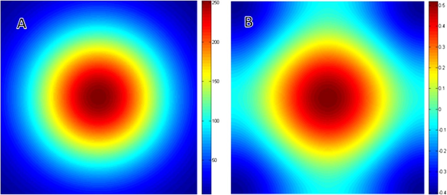
1. Introduction

Image correlation spectroscopy (ICS) has gained acceptance for its ability to quantitatively analyze fluorophore distribution in a user-independent manner from relatively noisy images. Originally described in 1993 using math from statistical mechanics,¹ it has since gained acceptance for analyzing biological macromolecule organization ( $> 100$ publications using the term in the title). ICS is especially adept at distinguishing images with a homogeneous fluorophore (macromolecule) distribution from those with the same mean intensity, but uneven, clustered fluorophore distribution in an automated and user-independent fashion. The ability to distinguish these two states is extremely useful in biological systems where clustering of macromolecules can differentiate cellular processes (e.g., receptor aggregation²^–⁴ and collagen fiber organization).⁵ ICS has since been extended to analyze fluorophore colocalization (cross correlation ICS),⁶^–⁸ dispersion and diffusion in time (spatiotemporal⁹^–¹¹ and raster ICS),¹²^–¹⁶ and macromolecular structure.⁵^,¹⁷ More information about these variants can be found in several recent reviews,⁶ showing the versatility of this mathematical technique.

ICS, in all its variants, relies on calculation of the image autocorrelation followed by a fit of the autocorrelation function to a two-dimensional (2-D) Gaussian function to extract quantitative parameters. Few previous works have analyzed the effects of image structure or artifacts on the fidelity of this process, and those that have rely heavily on simulations.¹⁷^,¹⁸ Both autocorrelation and Gaussian curve fitting can be analyzed analytically via estimation theory; however, no previous work has established the theory necessary or described the effect of imaging artifacts in this manner.

It is important to understand the mathematical theory underlying autocorrelation-based analysis for two reasons. Firstly, preprocessing, curve fitting, and noise reduction induce significant variance in ICS analyses. The lack of consensus in preprocessing and analysis makes comparing results across publications difficult, and may bias results. Secondly, the peak of the autocorrelation function is inversely related to particle number, modified by particle size and shape; however, the autocorrelation function also encodes further information about image structure. By expanding on autocorrelation theory, quantitative image analysis can be advanced. Instead of using simulations to model autocorrelation-based image analysis, we seek instead to analytically describe the effects of artifacts commonly seen in laser-based microscopy and image processing operations, followed by a series of practical recommendations that will provide greater uniformity and accuracy in applying ICS to fluorescent images.

2. Three Definitions of Autocorrelation

Autocorrelation itself is logically equivalent to comparing all possible pixel pairs and reporting the likelihood that both will be bright as a function of the distance and direction of separation. In a more mathematical definition, autocorrelation is the convolution of a function with itself. For a digital image $I$ , of size $M \times N$ (images are discretely spatially defined, 2- to 4-dimensional, of finite extent, and have real, bounded, digital values), autocorrelation can be calculated by Eq. (1)

Eq. (1)

G i i (a, b) = \sum_{x}^{M} \sum_{y}^{N} i (x, y) * i (x - a, y - b),

where

G i i (a, b)

is the autocorrelation function,

i (x, y)

is the image intensity at position

(x, y)

, and

a

and

b

represent the distance (or lag) from the corresponding

x

and

y

position. The analysis in this work assumes that the image is homogeneous (or ergodic). For example, if an image has boundaries like a cell on a background it should be cropped to be homogeneous. As the mean value and range of real digital images are based on acquisition system and parameters instead of the underlying structure, the normalized autocorrelation, denoted

g_{i i}

, is used for analyses such as ICS. It is calculated by dividing

G

by the square of the mean intensity and subtracting 1 from that quantity,

Eq. (2)

g i i (a, b) = \frac{\sum_{x}^{M} \sum_{y}^{N} i (x, y) * i (x - a, y - b)}{\sum_{x}^{M} \sum_{y}^{N} i (x, y) * i (x, y)} - 1 = \frac{F^{- 1} {F {[i (x, y)]}^{2}}}{N M i^{2}} - 1,

where

F (x, y)

is the Fourier transform of

i (x, y)

. For images which are isotropic (i.e., no orientation),

G i i

and

g i i

will be radially symmetric, which thus produces

g i i (d)

, where

d

is the length to

(a, b)

.

Practically, Eqs. (1) and (2) are almost never used; autocorrelations can be calculated far more efficiently via fast Fourier transforms using the Weiner-Khinchin theorem,

Eq. (3)

F^{- 1} [G i i (a, b)] = S (i) = {| F [i (x, y)] |}^{2},

where

S (i)

is the power spectrum of the image. This powerful theorem states that the Fourier transform of the autocorrelation of an image

i

is equal to the inverse Fourier transform of

S (i)

. The power spectrum can be calculated by squaring the magnitude of the Fourier transform of

i

, which for real-valued functions is equivalent to multiplying the Fourier transform by its converse. This theorem is important for two reasons. First, it reduces processing time [from

O = n^{4}

to

n \log (n)

], and, second, it links the autocorrelation operator to the more commonly understood (and blessedly linear) Fourier transform.

The last formulation for the autocorrelation operator we will use for this analysis is a heuristic formulation of the probability that two points will accord based on the vector between them. We will focus on the expected autocorrelations for image classes which are defined statistically (i.e., white noise with a certain spatial and intensity profile). For these image classes, autocorrelation can be understood as the product of the predicted intensity distribution of a pixel $[P_{i} (x, y)]$ in the image and the predicted intensity distribution of pixels a certain distance away $[P_{i} (x + a, y + b)]$ . This gives a predicted image autocorrelation, ${G p}_{i i}$ , and predicted normalized autocorrelation ${g p}_{i i}$ (assuming the probability density sums to 1),

Eq. (4)

{G p}_{i i} (a, b) = P_{i} (x, y) * P_{i} (x + a, y + b) and

Eq. (5)

{g p}_{i i} (a, b) = P_{i} (x, y) * P_{i} (x + a, y + b) - 1.

The normalized probability density function

(P_{i})

of a real image can be calculated by dividing the intensity distribution of the image by the sum of the image values, giving a probability function which sums to 1.

3. Creation of Test Images

Creating images to test new autocorrelation-based techniques requires understanding of the acquisition system that will be used for experimental images. Ideally these test images would be created on the acquisition system itself, in which case, the correct noise and point spread fuction (PSF) artifacts will already be part of the image. If this is not feasible, algorithms should be tested against test images with artificially created artifacts and blur of the same magnitude as expected in real images.

4. Effects of Common Artifacts and Processing Steps

4.1.

Scaling

Multiplication of all image values by a constant, impacts the autocorrelation nonlinearly: $G [k * i] = k^{2} * G [i]$ , but it does not affect the normalized autocorrelation $g$ , as $g = G / mean {(i)}^{2} = k^{2} G [i] / (k^{2} mean {(i)}^{2}) = g [i]$ . For digital images, scaling may improve autocorrelation fidelity as decimation errors are minimized. Empirically, scaling an image to use the entire range of the detector system will offer the best data fidelity.

4.2.

Linear Filtering

Linear filtering is defined by the convolution of image $i (x, y)$ with the discrete filter kernel $h$ , and is equivalent to (and normally calculated by) multiplying their Fourier transforms: $F^{- 1} [F (i) F (h)] = F^{- 1} [F (i)] * F^{- 1} [F (h)]$ . It is then trivial to see that applying a filter to an image before autocorrelation would be equivalent to convolving the autocorrelation of the image with the autocorrelation of the filter. From a practical point of view, if an image is filtered before autocorrelation is performed, roundoff error may be worth considering. Repeated transformations into Fourier space can degrade the image if bit-depth is insufficient.

Similarly, real optical systems have a finite (PSF, commonly modeled as a Gaussian function), which serves as a low-pass filter for the acquired image. Therefore, the autocorrelation of a confocal or multiphoton image will equal that of the true image convolved with the autocorrelation of the optical system point spread function. Convolving two radially symmetric 2-D Gaussians (with amplitudes $A 1$ and $A 2$ and deviations $s 1$ and $s 2$ ) in two dimensions results in a third Gaussian function with a standard deviation equal to $sqrt (s 1^{2} + s 2^{2} / s 1 * s 2)$ and amplitude $[A 1 * A 2 * (s 1^{2} + s 2^{2})]$ . If one standard deviation, say that of the optical system, is much larger than the other, it will tend to dominate the deviation of the resulting function. As a result, for images of small particles (smaller than the diffraction limit), the deviation of the Gaussian fit will relate to the PSF for confocal or multiphoton systems, limited by the spot size of the laser (laser beam waist).¹ On the other hand, this will not be the case for images which have broader autocorrelations, like images of fibers longer than the diffraction limit (see Sec. 5.4 on randomly oriented fibers). Comparing the standard deviation and the beam waist (or optical system point spread function) has been used in the past as a check on the processing fidelity. Thus, if the standard deviation from the Gaussian fit approximately equals the beam waist (i.e., a positive result) then acquisition and optimization are satifactory, but a negative result does not necessitate image rejection.

4.3.

Addition of Two Images

The importance of adding two images lies in the ability to model noise as an image added to the information-containing image. For Gaussian white noise [e.g., thermal fluctuations in a charge coupled device (CCD)], this assumption is commonly made and reasonably accurate. The autocorrelation of the superposition of two images $i (x, y)$ and $j (x, y)$ is

Eq. (6)

G_{i + j} = F^{- 1} [{| F (i + j) |}^{2}] = F^{- 1} [{| F (i) + F (j) |}^{2}] = F^{- 1} [{| F (i) |}^{2} + {| F (j) |}^{2} + | F (j) * \underset{̲}{F} (i) + F (i) * \underset{̲}{F} (j) |] = G_{i i} + G_{j j} + 2 * G_{i j} .

Therefore, the autocorrelation of the sum of two images is equal to the autocorrelation of each plus the convolution of image

i

with image

j

. If noise is added to an image, the autocorrelation of the noisy image will be affected both by the autocorrelation of the noise with itself and the convolution of the noise with the image. More details of the implications are described below in Sec. 5.2 on white noise.

4.4.

Thresholding

Thresholding reduces the intensity information of an image to 0 or 1, allowing use of binary image processing algorithms, and increasing the image contrast. Theoretically, thresholding should minimally affect the spatial distribution (which autocorrelation principally analyzes) of the image. By definition, it will alter the intensity probability density function, which will affect the scaling of the normalized autocorrelation. The maximum of the autocorrelation relates to both image structure and image probability distribution. A binary image has a mean intensity of one times the fraction of pixels which are bright. Once normalized, the thresholded image will result in a mean normalized probability distribution of 1. Any unthresholded image with a broad normalized intensity probability function would have a lower average. In theory, therefore, thresholding before autocorrelation could allow for analysis of spatial distribution independent of intensity.

In practice, thresholding will affect spatial distribution as well as normalized probability distribution. For example, thresholding will enhance the edges of images that have some finite intensity roll off (soft edges), serving as a high-pass filter. Depending on the threshold chosen, particle size may be over- or underestimated, which will affect the roll off of the autocorrelation function and its maximum value. In cases where thresholding is hard, (relatively poor signal to noise ratio or high background to signal ratio) thresholding may obviate the underlying signal. In experimental work, the threshold level was shown to greatly affect autocorrelation maximum.¹⁷ Likewise, if the image is relatively noisy, thresholding can amplify noise, reducing autocorrelation fidelity. For these reasons, thresholding before autocorrelation analysis should be done judiciously and documented well.

4.5.

Background Subtraction

Background subtraction is a nonlinear noise reduction technique. An image of an empty field is taken to assess the noise levels of the detector system, and the mean value of this noise is set to be the 0 value for actual images. This will ensure that the background of real images is close to zero, while maintaining the fidelity of information-containing regions.⁵ This technique is an inherently nonlinear technique (making it difficult to quantitatively analyze) that affects only relatively dark pixels. The effect should be relatively minimal, however, as bright pixels dominate the autocorrelation.

4.6.

Sampling

As digital images have defined pixel sizes, many of the concepts presented here will hold true only in a statistical sense. Smaller images are more likely to differ from statistical norms due to smaller sample size. Autocorrelation has been performed on image subsets down to $16 \times 16$ pixel size, however, this is not recommended. On the other hand, the region analyzed should be homogeneous. Edges (e.g., cell borders) will tend to dominate the Fourier transform and hence the autocorrelation. Thus, larger image regions minimize statistical deviations, with the caveat that the region should be homogeneous.

Lastly, for laser-based imaging techniques, if the image pixel size is greater than the laser beam waist, sampling will serve as a form of low-pass filtering. If the pixel size is less than the laser beam waist, then the laser itself will serve as the primary filter. Previous work has used the laser beam waist as an independent validation of the fitting process¹⁹; however, to do so the detector must oversample the field of view relative to the laser beam waist.

5. Autocorrelation of Example Image Classes

5.1.

Monochrome Field

A monochrome field image $i (x, y)$ is equal to a constant $k$ for all $x$ and $y$ . The power spectrum of a flat field is equal to the sum of the image at the origin and zero elsewhere (akin to the Dirac delta function). The inverse Fourier transform of this power spectrum is equal to zero, so the normalized autocorrelation will be a flat field. A monochrome image, $m$ , superimposed on an information containing image, $i$ , will not affect the autocorrelation of $I (g_{i + m})$ . That is, $g (i + m) = g_{i i} + g_{m m} + 2 * g_{i m} = g_{i i}$ , as $g_{m m} = 0$ and $g_{i m} = 0$ .

5.2.

White Noise

White noise is spatially random, which gives it an even power spectrum across all frequencies (i.e., $F [G i i] = constant$ ). White describes the spatial correlation of intensity, whereas the intensity distribution of any given pixel can vary (e.g., Gaussian or Poisson). Many types of noise can be modeled as white, including background thermal noise (which is commonly modeled as Gaussian white noise.) An image comprised of white noise, by definition, has a flat power spectrum with a variance from the mean proportional to the intensity profile of the noise squared. A flat power spectrum will give a normalized autocorrelation equal to the Dirac delta function. In theory, therefore, ideal white noise will have an autocorrelation equal to zero everywhere but the origin. The value at the origin is equal to the normalized power spectrum squared. A value of 1 corresponds to “salt and pepper” noise; for Gaussian white noise the value will be the mean amplitude of the noise squared. (See Fig. 1.)

Fig. 1

Autocorrelation of Gaussian white noise. Frame (a) shows the original image and (b) its autocorrelation. The autocorrelation is very close to zero except at the origin.

When white noise is added to an information containing image, the autocorrelation of the resulting image should theoretically be unchanged. The autocorrelation of the information-containing image plus that of the white noise (equal to zero except at the origin), plus the convolution of the noise with the image (which should be similar to zero if the noise and the image are dissimilar) all sum to just the autocorrelation of the information-containing image: $g (i + m) = g_{i i} + g_{m m} + 2 * g_{i m} = g_{i i}$ , as $g_{m m} = 0$ except at the origin and $g_{i m} = 0$ as noise and the information containing image should be uncorrelated.

In practice, however, adding random noise to an image will blur the resulting autocorrelation. The values $g_{m m}$ and $g_{i m}$ are equal to zero only in a statistical sense: $g_{m m}$ has mean of 0 and a standard deviation related to the noise distribution. The correlation between the noise and the information containing image, $g_{i m}$ , should be close to zero for most image classes, though this depends on the information containing image. For these reasons it is important to acquire images with the best signal to noise ratio possible, and to omit the autocorrelation data at the origin from the Gaussian fits.

It should be noted that using low-pass filtering to reduce noise for autocorrelation analysis will adversely affect autocorrelation fidelity. Theoretically, the autocorrelation of white noise should be confined to the origin; however, low-pass filtering will artificially broaden $g_{m m}$ , the autocorrelation of the noise, which thus affects the curve fitting process. Lastly, it should be noted that for images of white noise, limited image size will increase the chance that the calculated autocorrelation will deviate from statistical norms (due to limited sample size). The mathematical framework described thus far deals with a representative image obeying statistical norms. Statistical chance may generate images which vary from the expected described above with likelihood inversely proportional to image size, once again highlighting the importance of acquiring appropriately large images.

5.3.

Gaussian Function

Gaussian functions are commonly used as low-pass filters or to model the point spread function of a laser. A 2-D Gaussian function centered at the origin with deviations in the $x$ and $y$ directions of $σ_{x}$ and $σ_{y}$ is defined by the equation $f (x, y) = \exp (- x^{2} / {σ_{x}}^{2} - y^{2} / {σ_{y}}^{2})$ . The autocorrelation of this function is another Gaussian: $G_{f f} (d) = π / (2 σ_{x} σ_{y}) * \exp (- x^{2} / 2 {σ_{x}}^{2} - y^{2} / {σ_{y}}^{2})$ , with smaller standard deviations and a different amplitude (Fig. 2). Since the integral of $G_{f f}$ over the whole real plane is $π * | σ_{x} σ_{y} |$ , the normalized autocorrelation $g_{f f} = 1 / (2 {σ x}^{2} {σ y}^{2}) * \exp (- x^{2} / 2 {σ_{x}}^{2} - y^{2} / {σ_{y}}^{2}) - 1$ . Note that this normalized autocorrelation is equal to $1 / (2 σ x^{2} σ y^{2})$ at the origin, and is equal to -1when $x$ or $y$ approach infinity.

Fig. 2

Autocorrelation of Gaussian functions. Frame (a) shows the original image and (b) shows its autocorrelation. While similar, some distortion can be seen in the autocorrelation. Note the scale on the original image goes from an intensity value of 0 to 255, and the autocorrelation from $- 0.5$ to 0.5.

5.4.

Randomly Dispersed and Randomly Oriented Fibers

This image will be comprised of randomly dispersed narrow fibers ( $n$ fibers per unit area) of length $L$ (and width of 1 pixel), all aligned randomly. To start, we will assume that the image is comprised of perfectly dark background pixels with evenly bright fibers. The probability of any pixel being part of fiber is therefore $P_{i} (x, y) = n * L$ . Given that the first pixel is part of a fiber, the probability that a second pixel at $(x + a, y + b)$ will also be part of the fiber is equal to the probability that the fiber lies in direction $(a, b)$ times the probability that if the fiber lies in the same direction, $(x + a, y + b)$ will not exceed the fiber’s length $L$ . $P i (x + a, y + b)$ therefore is equal to $(L - d) * 1 / 2 π d$ or $1 - 1 / 2 L d$ . For digital images, which are discretized, where the number of points $d$ pixels away from a center point is better modeled as $2 + 2 π * d$ (as opposed to $2 π d$ ). $P i (x a, y b)$ therefore becomes $1 / (1 + π d)$ . The image intensity is $n L$ which therefore gives the following predicted autocorrelation for digital images,

Eq. (7)

g i i (x, y) = \frac{1}{n L + n L π \sqrt{x^{2} + y^{2}}}

(See Fig. 3). If the center pixel

[g (0, 0)]

of this function is omitted, the Gaussian function fit will be underestimated, and underestimated more severely the more the peripheral regions of the autocorrelation are emphasized.

Fig. 3

Autocorrelation of randomly dispersed fibers. Frame (a) shows the test image and (b) its autocorrelation. Note the non-Gaussian profile of this image: the falloff is faster than Gaussian.

For a laser-based image, assuming no noise, the autocorrelation will equal $g i i$ of the information-containing image convolved with that of the optical system, which we will model as a Gaussian with deviation $w_{0}$ .The solution, while closed form, is not simple. We can state, however, that the autocorrelation of an information containing image convolved with a Gaussian beam has an autocorrelation which is not strictly Gaussian as the falloff in the central regions will be faster, and in the outlying regions slower. The peak of this function will equal $n L / {w_{0}}^{2}$ , however, as the falloff is faster than Gaussian, the fit will underestimate this value. If using ICS to analyze images of fibers, changes in number density and length will both affect the result, and $g (0, 0)$ will underestimate particle number.

6. Anisotropic Images

6.1.

Horizontal Lines of Random Intensity

The next image to be considered is anisotropic (i.e., image properties depend on orientation) characterized by parallel lines with random intensity. Note that this image is equivalent to a line of white noise, expanded horizontally to fill the image size. This anisotropic image will have an anisotropic autocorrelation: the central line of the autocorrelation, which evaluates the concordance of any two pixels on the horizontal line, will be maximal while the rest of the image will be zero. If we assume that this image of streaks is binary (i.e., it has been thresholded such that any pixel has a value of either 0 or 1), the value of the normalized autocorrelation along the horizontal axis will be 1. If we allow the value of the streaks to vary, the value along the horizontal axis will equal the mean of the normalized image intensity probability density function (since the probability that a first pixel will be bright is equal to $P n$ , and the probability that a pixel next to it will be bright is 1). If an image of horizontal white streaks is acquired with an optical system with a Gaussian point spread function, the resulting autocorrelation will have a Gaussian profile along the $y$ -axis (horizontal axis) with deviation equal to that of the optical point spread function.

6.2.

Aligned White Fibers

Autocorrelation is sensitive to alignment, as demonstrated in the horizontal lines of random intensity. To start, assume all fibers are equally bright, 1 pixel wide, have a length of $L$ and a density of $n$ fibers per area, and aligned horizontally. Unlike the previous case, the fibers in this image have a finite length of $L$ . The probability of a first point being part of a fiber is equal to $n * L$ , and the probability of a second point at a horizontal distance $x$ away being part of the same fiber is equal to $(L - x) / L$ . Note that if the direction of interest is not parallel to the horizontal the probability of that point also being part of a fiber is akin to the white noise scenario, e.g., equal to 0. The mean value of the image is $n * L$ , so after normalization the following equation is obtained

Eq. (8)

g i i (x, y) = {\begin{cases} L - x / {n L}^{2}, & x \leq L, y = 0 \\ 0, & x > L or y \neq 0 \end{cases} .

We can see that if we were to model this function with a 2-D Gaussian function, the standard deviation in the minor axis will approach zero, whereas in the major axis it will be proportional to

L

as noted in previous work that used simulations (Fig. 4).¹⁸

Fig. 4

Autocorrelation of aligned fibers. Frame (a) shows whitely distributed aligned fibers and frame (b) its autocorrelation. Note that the horizontal axis contains the only nonzero elements.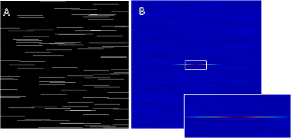

It is important to note that for images acquired with a real optical system, the deviation on the minor axis is bounded by that of the point spread function of the system. As such, reporting the ratio of the major and minor axis standard deviation (elipticity²⁰ or skew⁵) may be misleading. If the autocorrelation of the true image $i$ has uneven deviations ( $s_{x}$ and $s_{y}$ ) and is convolved with a radially symmetric Gaussian PSF with deviation $w$ , the resulting function will have uneven distributions equal to

Eq. (9)

g i i * g_{psf psf} = e^{- \frac{x^{2}}{{s_{x}}^{2}} - \frac{y^{2}}{{s_{y}}^{2}}} * e^{- \frac{(x^{2} + y^{2})}{w^{2}}} = e^{- \frac{s_{x} w x^{2}}{{s_{x}}^{2} + w^{2}} - \frac{s_{y} w y^{2}}{{s_{y}}^{2}}} .

Comparing deviation of the major and minor axes will give

\frac{s_{x}}{s_{y}} \sqrt{\frac{{s_{y}}^{2} + w^{2}}{{s_{x}}^{2} + w^{2}} .}

If

w

is small relative to

s_{y}

and

s_{x}

, ellipticity will be accurate, but if not, elipticity will not relate linearly to the ratio of

s_{x}

and

s_{y}

.

7. Curve Fitting

All ICS analysis uses nonlinear optimization to fit a 2-D Gaussian to the autocorrelation function, with wide variation in the method and equation used for fitting. Having described predicted image autocorrelations for several image classes, we can analytically describe some aspects of the curve fitting process and offer some recommendations. A full description of methods for Gaussian curve fitting is beyond the scope of this work (Refs. 21 and 22); nonetheless, we can provide a review of the strengths and weaknesses of previously published methods.

When ICS was first introduced in 1993, nonlinear optimization was time consuming and complicated, necessitating a reductionist approach. As a result, the autocorrelation was fit to 1-D Gaussian functions along the two axes only. More modern work crops the information-containing regions of the autocorrelation function and then fits the entire region to a 2-D Gaussian function. Cropping varies in different publications, ranging from the central $16 \times 16$ pixels to three times the laser beam width.²³ Likewise, several different Gaussian functions have been used, ranging from simple models which assume the same standard deviation in both $x$ and $y$ (see Ref. 1) to more complicated models which allow different deviations on the major and minor axes.²⁰ Despite these advances, accurate curve fitting remains tricky, given that several image classes have non-Gaussian autocorrelations.

7.1.

Cropping

Cropping speeds curve fitting and rejects regions with low signal to noise ratio. As processing power increases and user-friendly curve fitting packages become more widely dispersed, cropping for speed becomes less important. However, rejecting regions with low signal to noise remains a fundamental reason to consider cropping. If the autocorrelation of an image is Gaussian with some noise, the central regions with higher values will have higher signal to noise ratio. Likewise, points further from the center of the autocorrelation have a smaller signal to noise ratio, but there are more of these points which provides an intrinsic weighting of these points. Cropping reduces this intrinsic bias, which explains its widespread adoption.

For laser based images with Gaussian autocorrelations dominated by the laser point spread function, cropping to three times the radius of the point spread function will provide an image containing the useable data while rejecting the regions with low signal to noise.²³ However, most interesting images have structures larger than the laser point spread function in them (at least if the laser was correctly selected), which will lead to images with broader autocorrelations. Cropping at three times the beam waist will weight the fit to shorter standard deviations. For images that have non-Gaussian autocorrelations, such as the randomly oriented fibers case discussed above, the amplitude of the Gaussian will be higher for more severe cropping. Alternatives to cropping followed by fitting include maximum likelihood estimation fitting²¹^,²² and weighted least squares optimization.

7.2.

Gaussian Model

Early work was most interested in the amplitude alone of the function, and thus a simple equation assuming radial symmetry was used. More recent work, investigating either alignment or cross correlation, have used more complicated formulations of the Gaussian. A particularly attractive Gaussian form is,

Eq. (10)

g = A e^{a {(x - x_{0})}^{2} + b (x - x_{0}) (y - y_{0}) + c {(y - y_{0})}^{2}} + g_{0} .

This form copes with both center-misalignment and oriented images, but necessitates a seven parameter fit, which may be unwieldy. However, if the autocorrelation is known to be well-centered, $x_{0}$ and $y_{0}$ can be set a priori, which reduces the parameter space by two.

7.3.

Data Omission for Noise Reduction

As white noise exclusively affects the origin of the autocorrelation, the origin is normally omitted from the fit, as is the data from any known artifacts. If an image of a dark field is taken, the quantity and distribution of noise can be analyzed. Therefore it is good practice to acquire a blank image (picture of nothing) to determine system noise, and to use the autocorrelation of this image to inform artifact rejection.

Note that optimization of Eq. (10) is guaranteed to not be convex, which makes fitting difficult (as $- 90 \deg \sim 270 \deg$ , for example). One can either rely on constraints to minimize the parameter space to create a convex subspace, or work on creating good initial conditions to aid convergence. Empirically, good initial conditions are needed for efficient, correct optimization. Theoretically ideal initial conditions have been the subject of previous work.²⁴

8. Conclusions

Autocorrelation offers a tool to analyze image structure in a user-independent manner and has proven useful in analysis of several macromolecule systems. Given the variation in image preprocessing and autocorrelation analysis, we felt it necessary to describe the effects of several common processes and offer recommendations for greater uniformity and accuracy.

Acknowledgments

We would like to thank Enrico Gratton for his comments on this manuscript.

References

1.

N. O. Petersenet al., “Quantitation of membrane receptor distributions by image correlation spectroscopy: concept and application,” Biophys. J., 65 (3), 1135 –1146 (1993). http://dx.doi.org/10.1016/S0006-3495(93)81173-1 BIOJAU 0006-3495 Google Scholar

2.

T. SungkawornY. LenburyV. Chatsudthipong, “Oxidative stress increases angiotensin receptor type I responsiveness by increasing receptor degree of aggregation using image correlation spectroscopy,” Biochim. Biophys. Acta, 1808 (10), 2496 –2500 (2011). http://dx.doi.org/10.1016/j.bbamem.2011.07.007 BBACAQ 0006-3002 Google Scholar

3.

J. BonorA. Nohe, “Image correlation spectroscopy to define membrane dynamics,” Methods Mol. Biol., 591 353 –364 (2010). http://dx.doi.org/10.1007/978-1-60761-404-3 1064-3745 Google Scholar

4.

E. KeatingA. NoheN. O. Petersen, “Studies of distribution, location and dynamic properties of EGFR on the cell surface measured by image correlation spectroscopy,” Eur. Biophys. J., 37 (4), 469 –481 (2008). http://dx.doi.org/10.1007/s00249-007-0239-y EBJOE8 0175-7571 Google Scholar

5.

C. B. Raubet al., “Image correlation spectroscopy of multiphoton images correlates with collagen mechanical properties,” Biophys. J., 94 (6), 2361 –2373 (2008). http://dx.doi.org/10.1529/biophysj.107.120006 BIOJAU 0006-3495 Google Scholar

6.

D. L. KolinP. W. Wiseman, “Advances in image correlation spectroscopy: measuring number densities, aggregation states, and dynamics of fluorescently labeled macromolecules in cells,” Cell Biochem. Biophys., 49 (3), 141 –164 (2007). http://dx.doi.org/10.1007/s12013-007-9000-5 CBBIFV 1085-9195 Google Scholar

7.

J. V. RocheleauP. W. WisemanN. O. Petersen, “Isolation of bright aggregate fluctuations in a multipopulation image correlation spectroscopy system using intensity subtraction,” Biophys. J., 84 (6), 4011 –4022 (2003). http://dx.doi.org/10.1016/S0006-3495(03)75127-3 BIOJAU 0006-3495 Google Scholar

8.

S. Semrauet al., “Quantification of biological interactions with particle image cross-correlation spectroscopy (PICCS),” Biophys. J., 100 (7), 1810 –1818 (2011). http://dx.doi.org/10.1016/j.bpj.2010.12.3746 BIOJAU 0006-3495 Google Scholar

9.

J. Boveet al., “Magnitude and direction of vesicle dynamics in growing pollen tubes using spatiotemporal image correlation spectroscopy and fluorescence recovery after photobleaching,” Plant Physiol., 147 (4), 1646 –1658 (2008). http://dx.doi.org/10.1104/pp.108.120212 PLPHAY 0032-0889 Google Scholar

10.

B. HebertS. CostantinoP. W. Wiseman, “Spatiotemporal image correlation spectroscopy (STICS) theory, verification, and application to protein velocity mapping in living CHO cells,” Biophys. J., 88 (5), 3601 –3614 (2005). http://dx.doi.org/10.1529/biophysj.104.054874 BIOJAU 0006-3495 Google Scholar

11.

M. RossowW. W. MantulinE. Gratton, “Spatiotemporal image correlation spectroscopy measurements of flow demonstrated in microfluidic channels,” J. Biomed. Opt., 14 (2), 024014 (2009). http://dx.doi.org/10.1117/1.3088203 JBOPFO 1083-3668 Google Scholar

12.

C. M. Brownet al., “Raster image correlation spectroscopy (RICS) for measuring fast protein dynamics and concentrations with a commercial laser scanning confocal microscope,” J. Microsc., 229 (1), 78 –91 (2008). http://dx.doi.org/10.1111/jmi.2008.229.issue-1 JMICAR 0022-2720 Google Scholar

13.

E. Gielenet al., “Measuring diffusion of lipid-like probes in artificial and natural membranes by raster image correlation spectroscopy (RICS): use of a commercial laser-scanning microscope with analog detection,” Langmuir, 25 (9), 5209 –5218 (2009). http://dx.doi.org/10.1021/la8040538 LANGD5 0743-7463 Google Scholar

14.

S. C. Norriset al., “Raster image correlation spectroscopy as a novel tool to study interactions of macromolecules with nanofiber scaffolds,” Acta Biomaterilas, 7 (12), 4195 –4203 (2011). Google Scholar

15.

M. J. Rossowet al., “Raster image correlation spectroscopy in live cells,” Nat. Protoc., 5 (11), 1761 –1774 (2010). http://dx.doi.org/10.1038/nprot.2010.122 NPARDW 1750-2799 Google Scholar

16.

M. VendelinR. Birkedal, “Anisotropic diffusion of fluorescently labeled ATP in rat cardiomyocytes determined by raster image correlation spectroscopy,” Am. J. Physiol. Cell Physiol., 295 (5), C1302 –1315 (2008). http://dx.doi.org/10.1152/ajpcell.00313.2008 0363-6143 Google Scholar

17.

P. W. Wisemanet al., “Counting dendritic spines in brain tissue slices by image correlation spectroscopy analysis,” J. Microsc., 205 (2), 177 –186 (2002). http://dx.doi.org/10.1046/j.0022-2720.2001.00985.x JMICAR 0022-2720 Google Scholar

18.

S. Costantinoet al., “Accuracy and dynamic range of spatial image correlation and cross-correlation spectroscopy,” Biophys. J., 89 (2), 1251 –1260 (2005). http://dx.doi.org/10.1529/biophysj.104.057364 BIOJAU 0006-3495 Google Scholar

19.

A. M. PetersenB. K. Pedersen, “The role of IL-6 in mediating the anti-inflammatory effects of exercise,” J. Physiol. Pharmacol., 57 (10), 43 –51 (2006). JPHPEI 0867-5910 Google Scholar

20.

S. M. MirB. BaggettU. Utzinger, “The efficacy of image correlation spectroscopy for characterization of the extracellular matrix,” Biomed. Opt. Express, 3 (2), 215 –224 (2012). http://dx.doi.org/10.1364/BOE.3.000215 BOEICL 2156-7085 Google Scholar

21.

N. HagenE. L. Dereniak, “Gaussian profile estimation in two dimensions,” Appl. Opt., 47 (36), 6842 –6851 (2008). http://dx.doi.org/10.1364/AO.47.006842 APOPAI 0003-6935 Google Scholar

22.

N. HagenM. KupinskiE. L. Dereniak, “Gaussian profile estimation in one dimension,” Appl. Opt., 46 (22), 5374 –5383 (2007). http://dx.doi.org/10.1364/AO.46.005374 APOPAI 0003-6935 Google Scholar

23.

A. NoheN. O. Petersen, “Image correlation spectroscopy,” Sci. STKE, 2007 (417), l7 –33 (2007). http://dx.doi.org/10.1126/stke.4172007pl7 Google Scholar

24.

D. JukićR. Scitovski, “Least squares fittingGaussian type curve,” Appl. Math. Comput., 167 (1), 286 –298 (2005). http://dx.doi.org/10.1016/j.amc.2004.06.084 AMHCBQ 0096-3003 Google Scholar

Citation Download Citation

Claire Robertson and Steven C. George M.D. "Theory and practical recommendations for autocorrelation-based image correlation spectroscopy," Journal of Biomedical Optics 17(8), 080801 (8 August 2012). https://doi.org/10.1117/1.JBO.17.8.080801

Published: 8 August 2012

Access the abstract

JOURNAL ARTICLE
8 PAGES

DOWNLOAD PAPER SAVE TO MY LIBRARY

GET CITATION

CITATIONS

Cited by 55 scholarly publications and 1 patent.

Explore citations on Lens.org

RIGHTS & PERMISSIONS

Get copyright permission Get copyright permission on Copyright Marketplace

KEYWORDS

Point spread functions

Image processing

Fourier transforms

Image analysis

Digital imaging

Image filtering

Imaging spectroscopy

1.

Introduction

2.

Three Definitions of Autocorrelation

Eq. (1)

Eq. (2)

Eq. (3)

Eq. (4)

Eq. (5)

3.

Creation of Test Images

4.

Effects of Common Artifacts and Processing Steps

4.1.

Scaling

4.2.

Linear Filtering

4.3.

Addition of Two Images

Eq. (6)

4.4.

Thresholding

4.5.

Background Subtraction

4.6.

Sampling

5.

Autocorrelation of Example Image Classes

5.1.

Monochrome Field

5.2.

White Noise

Fig. 1

5.3.

Gaussian Function

Fig. 2

5.4.

Randomly Dispersed and Randomly Oriented Fibers

Eq. (7)

Fig. 3

6.

Anisotropic Images

6.1.

Horizontal Lines of Random Intensity

6.2.

Aligned White Fibers

Eq. (8)

Fig. 4

Eq. (9)

7.

Curve Fitting

7.1.

Cropping

7.2.

Gaussian Model

Eq. (10)

7.3.

Data Omission for Noise Reduction

8.

Conclusions

Acknowledgments

References

Show All Keywords

Keywords/Phrases

Search In:

Publication Years