Extraction of effective parameters of turbid media utilizing the Mueller matrix approach: study of glucose sensing

Thi-Thu-Hien Pham; Yu-Lung Lo

doi:10.1117/1.JBO.17.9.097002

6 September 2012 Extraction of effective parameters of turbid media utilizing the Mueller matrix approach: study of glucose sensing

Thi-Thu-Hien Pham, Yu-Lung Lo

Author Affiliations +

Journal of Biomedical Optics, Vol. 17, Issue 9, 097002 (September 2012). https://doi.org/10.1117/1.JBO.17.9.097002

Abstract

An analytical technique based on Stokes polarimetry and the Mueller matrix method is proposed for extracting the effective linear birefringence, linear dichroism, circular birefringence, circular dichroism, linear depolarization, and circular depolarization properties of turbid media. In contrast to existing analytical models, the model proposed extracts the effective parameters in a decoupled manner and considers not only the circular dichroism properties of the sample, but also the depolarization properties. The results show that the proposed method enables all of the effective parameters to be measured over the full range. Moreover, it is shown that the extracted value of the depolarization index is unaffected by the order in which the depolarizing Mueller matrix is decomposed during the extraction procedure. Finally, a method is proposed for calibrating the optical rotation angle of a polystyrene microsphere suspension containing dissolved D-glucose (C₆H 1₂O₆ ) powder in accordance with the distance between the sample and the detector. The experimental results show that the sensitivity of the resulting D-glucose measurement is equal to approximately 1.73 deg/M .

1. Introduction

The polarization properties of scattered light from turbid media, such as biological tissues, human or animal muscle, and certain plastics, have received considerable attention due to their potential for use in inspection or diagnostic detection applications. Many different methodologies have been proposed for determining the optical properties of turbid media. For example, Prahl et al. proposed two methods based on a single-integrating-sphere system¹^,² and a double-integrating sphere system,³ respectively, for measuring the absorption coefficient, scattering coefficient and anisotropy factor of bovine muscle, human tissue and polyurethane. Broadly speaking, the methods presented in the literature for measuring the absorption coefficient and scattering coefficient of tissue are based on either time-domain diffuse reflectance,⁴^–⁷ frequency-domain diffuse reflectance,⁸^–¹⁰ spatially resolved steady-state diffuse reﬂectance,¹¹^,¹² optoacoustics,¹³ or digital micro-radiography.¹⁴

Cameron et al.¹⁵^–¹⁷ proposed a method based on a Mueller matrix imaging approach for estimating the scattering coefficient of turbid media, such as rat tissue and melanoma-based tissue culture. Luo and his group¹⁸^,¹⁹ used an effective Mueller matrix approach to characterize the spatially-resolved diffuse back-scattering patterns of highly scattered media based on the assumption that the photon trajectories include only three scattering events. A good agreement was observed between the back-scattering patterns obtained using the proposed method for a polystyrene sphere suspension and those obtained via Monte Carlo simulations. Wang et al.²⁰^,²¹ compared the back-scattering patterns of birefringent anisotropic turbid media obtained using a single-scattering model and a double-scattering model, respectively, with those obtained from Monte Carlo simulations. Ghosh et al.²²^–²⁵ proposed an approach based on the Mueller matrix polar decomposition method²⁶ for extracting the linear birefringence (LB), circular birefringence (CB), linear dichroism (LD), and depolarization coefficient of complex turbid media such as polyacrylamide phantoms, polystyrene microsphere suspensions, and sucrose. The validity of the proposed approach was demonstrated by means of Monte Carlo simulations.

Although the methods presented in Refs. 15 16.17.18.19.20.21.22.23.24.–25 provide a useful insight into the scattering behavior of turbid media, they have several significant drawbacks. For example, the methods proposed in Refs. 15 16.17.18.19.20.–21 are unable to measure enough properties of scattering media. Similarly, the methods presented in Refs. 22 23.24.–25 fail when the Mueller matrix of LD is singular. Azzam²⁷ proposed a differential Mueller matrix formalism for analyzing the propagation of partially-polarized light through anisotropic media. Ossikovski²⁸ extended the differential matrix formalism to the case of depolarizing media. Ortega-Quijano and Arce-Diego²⁹^,³⁰ proposed a differential Mueller matrix-based approach for measuring the optical properties of general depolarizing media in both the transmission and reflectance mode. However, the differential matrix formalism cannot be applied if the eigenvalue of the Mueller matrix has a nonpositive real value. Moreover, methods based on the differential matrix formalism are unable to provide full-range measurements of all the optical parameters.

In a recent study, Pham and Lo³¹ proposed a decoupled analytical technique for extracting the six effective LB, LD, CB and circular dichroism (CD) parameters of anisotropic optical materials. By decoupling the extraction process, the “multiple solutions” problem inherent in previous models³²^,³³ was avoided. However, the method was unable to extract the linear depolarization (L-Dep) and circular depolarization (C-Dep) properties of turbid samples. Accordingly, in the present study, an enhanced analytical model is proposed for extracting all the effective LB, CB, LD, CD, L-Dep and C-Dep parameters of a turbid medium in a decoupled manner. The validity of the proposed method is demonstrated by extracting the parameters of various optical samples. In addition, a method is proposed for calibrating the CB measurements of a polystyrene microsphere suspension containing dissolved D-glucose powder in accordance with the distance between the sample and the detector.

2. Proposed Analytical Model for Extracting Nine Effective Optical Parameters of Turbid Media

This section introduces the analytical model proposed in this study for determining the effective LB, LD, CB, CD, L-Dep, and C-Dep properties of a turbid medium. As shown in Fig. 1, in developing the optically equivalent model of the anisotropic material, the CD and LD components of the sample are assumed to be in front of the CB and LB components, which are in turn in front of the C-Dep and L-Dep components.³¹^–³³ The Mueller matrices for a LB material, LD material and CD material, respectively, can all be found in the Refs. 31 32.–33. The most general expression for a depolarizer can be expressed as:²⁶^,³⁴

Eq. (1)

M_{Δ} = [\begin{matrix} 1 & {0⃗}^{T} \\ {P⃗}^{T} & m_{Δ} \end{matrix}],

where

m_{Δ}

is a

3 \times 3

symmetric matrix;

{\vec{P}}^{T}

is a polarizance vector. However, according to the experimental results in Refs. 22 23.24.–25 and simplification of the analytical model, the Mueller matrix for a nonuniform depolarizing material can be expressed as

Eq. (2)

M_{Δ} = [\begin{matrix} 1 & 0 & 0 & 0 \\ p_{1} & e_{1} & 0 & 0 \\ p_{2} & 0 & e_{2} & 0 \\ p_{3} & 0 & 0 & e_{3} \end{matrix}] and | e_{1} |, | e_{2} |, | e_{3} | \leq 1,

where

p_{1}

,

p_{2}

and

p_{3}

are the elements of the polarizance vector (

{\vec{P}}^{T}

),

e_{1}

and

e_{2}

are the degrees of L-Dep; and

e_{3}

is the degree of circular depolarization. In general, the degree of depolarization can be quantified by the depolarization index,

Δ

, which has a value of 0 for a nondepolarizer and 1 for an ideal depolarizer.³⁵ According to Ref. 34, the depolarization index can be expressed as

Eq. (3)

Δ = 1 - \sqrt{\frac{\sum_{i = 1 \sim 3} e_{i}^{2}}{3}}, 0 \leq Δ \leq 1 .

Fig. 1

Schematic illustration of experimental setup used to extract LB, CB, LD, CD, L-Dep and C-Dep parameters of turbid optical sample.

It is noted that Eq. (3) is calculated when the first element of matrix $M_{Δ}$ given in Eq. (2) has a value of 1.

In summary, for a turbid medium with hybrid optical properties, a total of nine effective parameters should be extracted, namely the LB orientation angle ( $α$ ), the retardance ( $β$ ), the optical rotation angle ( $γ$ ), the LD orientation angle ( $θ_{d}$ ), the LD (D), the CD (R), the degrees of L-Dep ( $e_{1}$ and $e_{2}$ ), and the degree of circular depolarization ( $e_{3}$ ). Table 1 summarizes the notations, ranges and definitions of the nine effective parameters and the depolarization index, respectively.³⁶^,³⁷

Table 1

Symbols, ranges and definitions of effective parameters of turbid media with hybrid properties. 36,37

Name	Symbol	Range	Definition^a
Orientation angle of fast axis of LB	A	$0 \deg \sim 180 \deg$
Linear birefringence of LB	B	$0 \deg \sim 360 \deg$	$2 π (n_{s} - n_{f}) l / λ_{0}$
Optical rotation of CB	$Γ$	$0 \deg \sim 180 \deg$	$2 π (n_{-} - n_{+}) l / λ_{0}$
Orientation angle of LD	$θ_{d}$	$0 \deg \sim 180 \deg$
Linear dichroism of LD	$D$	$0 \sim 1$	$2 π (μ_{s} - μ_{f}) l / λ_{0}$
Circular dichroism of CD	$R$	$- 1 \sim 1$	$2 π (μ_{-} - μ_{+}) l / λ_{0}$
Linear depolarization	$e_{1}$ and $e_{2}$	$- 1 \sim 1$
Circular depolarization	$e_{3}$	$- 1 \sim 1$
Depolarization index	$Δ$	$0 \sim 1$

^an is refractive index, μ is absorption coefficient, l is path length through medium (thickness of material), and λ0 is vacuum wavelength. Furthermore, subscripts f and s represent the fast and slow linearly polarized waves, respectively, when neglecting the circular effects. Finally, + and − represent the right and left circular polarized waves, respectively, when neglecting the linear effects.

Figure 1 presents a schematic illustration of the model experimental set-up proposed in this study for characterizing the effective LB, LD, CB, CD, L-Dep and C-Dep properties of a turbid sample. As shown, the equipment includes a Helium-Neon (He-Ne) laser, a Stokes polarimeter, a polarizer (P) and a quarter-wave plate (Q) used to produce various linear and right- and/or left- handed circular polarization lights.

The output Stokes vector $S_{c}$ in Fig. 1 can be calculated as

Eq. (4)

S_{c} = {[\begin{matrix} S_{0} \\ S_{1} \\ S_{2} \\ S_{3} \end{matrix}]}_{c} = [M_{Δ}] [M_{l b}] [M_{c b}] [M_{l d}] [M_{c d}] {\hat{S}}_{c} = {(\begin{matrix} m_{11} & m_{12} & m_{13} & m_{14} \\ m_{21} & m_{22} & m_{23} & m_{24} \\ m_{31} & m_{32} & m_{33} & m_{34} \\ m_{41} & m_{42} & m_{43} & m_{44} \end{matrix}) (\begin{matrix} {\hat{S}}_{0} \\ {\hat{S}}_{1} \\ {\hat{S}}_{2} \\ {\hat{S}}_{3} \end{matrix})}_{c},

where

[M_{Δ}]

,

[M_{l b}]

,

[M_{c b}]

,

[M_{l d}]

, and

[M_{c d}]

are the effective Mueller matrices describing the depolarization, LB, CB, LD and CD properties of the turbid sample, respectively, and

{\hat{S}}_{c}

is the input Stokes vector. In the methodology proposed in this study, the sample is illuminated by six input polarization lights, namely four linear polarization lights (i.e.,

{\hat{S}}_{0 \deg} = {[\begin{matrix} 1, & 1, & 0, & 0 \end{matrix}]}^{T}

,

{\hat{S}}_{45 \deg} = {[\begin{matrix} 1, & 0, & 1, & 0 \end{matrix}]}^{T}

,

{\hat{S}}_{90 \deg} = {[\begin{matrix} 1, & - 1, & 0, & 0 \end{matrix}]}^{T}

, and

{\hat{S}}_{135 \deg} = {[\begin{matrix} 1, & 0, & - 1, & 0 \end{matrix}]}^{T}

) and two circular polarization lights (i.e., right-handed

{\hat{S}}_{RHC} = {[\begin{matrix} 1, & 0, & 0, & 1 \end{matrix}]}^{T}

and left-handed

{\hat{S}}_{LHC} = {[\begin{matrix} 1, & 0, & 0, & - 1 \end{matrix}]}^{T}

). The corresponding output Stokes vectors can be obtained from Eq. (4) as follows:

Eq. (5)

S_{0 \deg} = {[\begin{matrix} m_{11} + m_{12}, & m_{21} + m_{22}, & m_{31} + m_{32}, & m_{41} + m_{42} \end{matrix}]}^{T}

Eq. (6)

S_{45 \deg} = {[\begin{matrix} m_{11} + m_{13}, & m_{21} + m_{23}, & m_{31} + m_{33}, & m_{41} + m_{43} \end{matrix}]}^{T}

Eq. (7)

S_{90 \deg} = {[\begin{matrix} m_{11} - m_{12}, & m_{21} - m_{22}, & m_{31} - m_{32}, & m_{41} - m_{42} \end{matrix}]}^{T}

Eq. (8)

S_{135 \deg} = {[\begin{matrix} m_{11} - m_{13}, & m_{21} - m_{23}, & m_{31} - m_{33}, & m_{41} - m_{43} \end{matrix}]}^{T}

Eq. (9)

S_{RHC} = {[\begin{matrix} m_{11} + m_{14}, & m_{21} + m_{24}, & m_{31} + m_{34}, & m_{41} + m_{44} \end{matrix}]}^{T}

Eq. (10)

S_{LHC} = {[\begin{matrix} m_{11} - m_{14}, & m_{21} - m_{24}, & m_{31} - m_{34}, & m_{41} - m_{44} \end{matrix}]}^{T} .

Equations (5) to (10) are sufficient to calculate all of the elements of the Mueller matrix product given in Eq. (4) (i.e.,

m_{11} \sim m_{44}

. For simplicity, the LD and CD properties of the sample are computed using only elements

m_{11}

,

m_{12}

,

m_{13}

and

m_{14}

in Eq. (4). Specifically, the LD orientation angle (

θ_{d}

) is obtained as

Eq. (11)

2 θ_{d} = \tan^{- 1} [\frac{S_{45 \deg} (S_{0}) - S_{135 \deg} (S_{0})}{S_{0 \deg} (S_{0}) - S_{90 \deg} (S_{0})}] .

The LD (D) is obtained as

Eq. (12)

D = \sqrt{\frac{{[S_{0 \deg} (S_{0}) - S_{90 \deg} (S_{0})]}^{2} + {[S_{45 \deg} (S_{0}) - S_{135 \deg} (S_{0})]}^{2}}{{[S_{0 \deg} (S_{0}) + S_{90 \deg} (S_{0})]}^{2} - {[S_{RHC} (S_{0}) - S_{LHC} (S_{0})]}^{2}}}

or

Eq. (13)

D = \frac{[S_{0 \deg} (S_{0}) - S_{90 \deg} (S_{0})]}{\cos (2 θ_{d}) {\sqrt{{[S_{0 \deg} (S_{0}) + S_{90 \deg} (S_{0})]}^{2} - {[S_{RHC} (S_{0}) - S_{LHC} (S_{0})]}^{2}}}}

or

Eq. (14)

D = \frac{[S_{45 \deg} (S_{0}) - S_{135 \deg} (S_{0})]}{\sin (2 θ_{d}) {\sqrt{{[S_{0 \deg} (S_{0}) + S_{90 \deg} (S_{0})]}^{2} - {[S_{RHC} (S_{0}) - S_{LHC} (S_{0})]}^{2}}}} .

The CD (

R

) is obtained as

Eq. (15)

R = \frac{[S_{0 \deg} (S_{0}) + S_{90 \deg} (S_{0})] - {\sqrt{{[S_{0 \deg} (S_{0}) + S_{90 \deg} (S_{0})]}^{2} - {[S_{RHC} (S_{0}) - S_{LHC} (S_{0})]}^{2}}}}{[S_{RHC} (S_{0}) - S_{LHC} (S_{0})]} .

Significantly, the values of

θ_{d}

,

D

, and

R

obtained from Eqs. (11), (12), and (15), respectively, are decoupled from one another. That is,

θ_{d}

can be determined with no prior knowledge of

D

or

R

,

D

can be derived with no knowledge of

θ_{d}

or

R

, and

R

can be computed with no knowledge of

θ_{d}

or

D

. Moreover, for values of

θ_{d}

other than 0 deg or 45 deg, Eqs. (12) through (14) yield the same theoretical solution, and thus the equality (or otherwise) of the results obtained from the three equations provides the means to check the correctness of the experimental results.

Once the LD and CD properties are known, the product of the LD and CD Mueller matrices can be calculated as

Eq. (16)

M_{D} = [M_{l d}] [M_{c d}] = (\begin{matrix} B_{11} & B_{12} & B_{13} & B_{14} \\ B_{12} & B_{22} & B_{23} & B_{24} \\ B_{13} & B_{23} & B_{33} & B_{34} \\ B_{41} & B_{42} & B_{43} & B_{44} \end{matrix}),

where

B_{11}

to

B_{44}

are all functions of

θ_{d}

,

D

and

R

, and can be extracted from Eqs. (11), (12), and (15), respectively. Note that all of the elements in the matrix product other than

B_{42}

and

B_{43}

are nonzero. The Mueller matrix of retardance has the form

Eq. (17)

M_{R} = [M_{l b}] [M_{c b}] = (\begin{matrix} 1 & A_{12} & A_{13} & A_{14} \\ A_{21} & A_{22} & A_{23} & A_{24} \\ A_{31} & A_{32} & A_{33} & A_{34} \\ A_{41} & A_{42} & A_{43} & A_{44} \end{matrix}),

where

A_{12}

through

A_{44}

are functions of the LB orientation angle (

α

), phase retardance (

β

) and CB optical rotation angle (

γ

). It is noted that elements

A_{12}

,

A_{13}

,

A_{14}

,

A_{21}

,

A_{31}

and

A_{41}

in Eq. (17) are all equal to zero. The Mueller matrix product

[M_{Δ \cdot R}]

can be expressed as

Eq. (18)

M_{Δ \cdot R} = [M_{Δ}] [M_{l b}] [M_{c b}] = (\begin{matrix} 1 & 0 & 0 & 0 \\ p_{1} & e_{1} A_{22} & e_{1} A_{23} & e_{1} A_{24} \\ p_{2} & e_{2} A_{32} & e_{2} A_{33} & e_{2} A_{34} \\ p_{3} & e_{3} A_{42} & e_{3} A_{43} & e_{3} A_{44} \end{matrix}) = (\begin{matrix} n_{11} & n_{12} & n_{13} & n_{14} \\ n_{21} & n_{22} & n_{23} & n_{24} \\ n_{31} & n_{32} & n_{33} & n_{34} \\ n_{41} & n_{41} & n_{43} & n_{44} \end{matrix}),

where all of the elements other than

n_{12}

,

n_{13}

, and

n_{14}

are nonzero.

From Eqs. (2), (4), (16), (17), and (18), the effective Mueller matrix corresponding to the LD, LB, CB, CD, L-Dep and C-Dep properties of the turbid optical sample can be expressed as

Eq. (19)

M_{Δ \cdot R \cdot D} = (\begin{matrix} B_{11} & B_{12} & B_{13} & B_{14} \\ n_{21} B_{11} + n_{22} B_{12} + n_{23} B_{13} + n_{24} B_{41} & n_{21} B_{12} + n_{22} B_{22} + n_{23} B_{23} & n_{21} B_{13} + n_{22} B_{23} + n_{23} B_{33} & n_{21} B_{14} + n_{22} B_{24} + n_{23} B_{34} + n_{24} B_{44} \\ n_{31} B_{11} + n_{32} B_{12} + n_{33} B_{13} + n_{34} B_{41} & n_{31} B_{12} + n_{32} B_{22} + n_{33} B_{23} & n_{31} B_{13} + n_{32} B_{23} + n_{33} B_{33} & n_{31} B_{14} + n_{32} B_{24} + n_{33} B_{34} + n_{34} B_{44} \\ n_{41} B_{11} + n_{42} B_{12} + n_{43} B_{13} + n_{44} B_{41} & n_{41} B_{12} + n_{42} B_{22} + n_{43} B_{23} & n_{41} B_{13} + n_{42} B_{23} + n_{43} B_{33} & n_{41} B_{14} + n_{42} B_{24} + n_{43} B_{34} + n_{44} B_{44} \end{matrix}) .

It is noted that all of the elements in matrix [ $M_{Δ \cdot R \cdot D}$ ] can be obtained from Eqs. (5) to (10) (i.e., from the experimental output Stokes vectors). In practice, once the elements in [ $M_{D}$ ] and [ $M_{Δ \cdot R \cdot D}$ ] have been determined from Eqs. (5) to (10), the elements in [ $M_{Δ \cdot R}$ ] can be inversely derived.

In this study, two methods are proposed for calculating the LB and CB properties of a turbid optical sample. It is noted that the second separate method is presented for the particular case in which the LD is close to one. In the first method (the default method), the polarizance vector ${\vec{P}}_{Δ} (p_{1}, p_{2}, p_{3})$ , the degrees of linear and circular depolarization ( $e_{1}$ , $e_{2}$ and $e_{3}$ ), the LB orientation angle ( $α$ ), the phase retardance ( $β$ ), and the optical rotation angle ( $γ$ ) are derived utilizing the known elements $n_{i j}$ in matrix [ $M_{Δ \cdot R}$ ]. Specifically, the polarizance vector is obtained as

Eq. (20)

{\vec{P}}_{Δ} = [\begin{matrix} p_{1} \\ p_{2} \\ p_{3} \end{matrix}] = [\begin{matrix} n_{21} \\ n_{31} \\ n_{41} \end{matrix}] .

Meanwhile, the phase retardance (

β

) is obtained as

Eq. (21)

β = \cos^{- 1} [\sqrt{\frac{- (n_{22} n_{42} + n_{23} n_{43}) (n_{32} n_{42} + n_{33} n_{43})}{(n_{22} n_{43} - n_{23} n_{42}) (n_{32} n_{43} - n_{33} n_{42})}}]

or

Eq. (22)

β = \tan^{- 1} [\frac{n_{43}}{\cos (2 α + 2 γ) n_{44}}],

where

Eq. (23)

2 α + 2 γ = \tan^{- 1} (- \frac{n_{42}}{n_{43}}) .

It should be noted that in Eq. (22),

β

is decoupled from

α

and

γ

since the numerator, i.e.,

n_{43}

, contains the term

\cos (2 α + 2 γ)

, which is canceled out by the corresponding term in the denominator. In other words, the extracted values of the retardance axis angle and optical rotation angle, respectively, have no effect on the extracted value of the retardance. Subsequently, the LB orientation angle can be obtained as

Eq. (24)

α = \frac{1}{2} \tan^{- 1} [\frac{- (n_{22} n_{42} + n_{23} n_{43})}{\cos (β) (n_{22} n_{43} - n_{23} n_{42})}],

or

Eq. (25)

α = \frac{1}{2} \tan^{- 1} [\frac{\cos (β) (n_{32} n_{43} - n_{33} n_{42})}{n_{32} n_{42} + n_{33} n_{43}}] .

Importantly, in Eq. (24), $α$ is decoupled from $β$ since the term $\cos (β)$ appears in both the numerator and the denominator and is therefore canceled out. [Note that the same situation applies in Eq. (25).]

The optical rotation angle, $γ$ , can be obtained as

Eq. (26)

γ = \frac{1}{2} \tan^{- 1} (\frac{- C_{2} n_{22} + C_{1} n_{23}}{C_{1} n_{22} + C_{2} n_{23}})

or

Eq. (27)

γ = \frac{1}{2} \tan^{- 1} (\frac{- C_{3} n_{22} + C_{2} n_{23}}{C_{2} n_{22} + C_{3} n_{23}}),

where

Eq. (28)

C_{1} = \cos^{2} (2 α) + \cos (β) \sin^{2} (2 α)

Eq. (29)

C_{2} = \cos (2 α) (1 - \cos (β)) \sin (2 α)

Eq. (30)

C_{3} = \cos^{2} (2 α) \cos (β) + \sin^{2} (2 α) .

It is noted that in Eqs. (26) and (27), $γ$ is decoupled from $α$ and $β$ since the functions involving $α$ and $β$ [i.e., Eqs. (28) to (30)] appear in both the numerator and the denominator. The optical rotation angle can also be obtained as

Eq. (31)

γ = \frac{1}{2} \tan^{- 1} (- \frac{n_{42}}{n_{43}}) - α .

Note that in this case,

γ

is coupled with

α

. Nonetheless, Eq. (31) provides a useful means of verifying the correctness of the experimental result obtained using Eqs. (26) or (27).

The degrees of linear and circular depolarization can be obtained as

Eq. (32)

e_{1} = \frac{n_{22}}{A_{22}},

Eq. (33)

e_{2} = \frac{n_{33}}{A_{33}},

Eq. (34)

e_{3} = \frac{n_{44}}{A_{44}},

where

Eq. (35)

A_{22} = - \cos (2 α) [1 - \cos (β)] \sin (2 α) \sin (2 γ) + [\cos^{2} (2 α) + \cos (β) \sin^{2} (2 α)] \cos (2 γ),

Eq. (36)

A_{33} = \cos (2 α) [1 - \cos (β)] \sin (2 α) \sin (2 γ) + [\cos^{2} (2 α) \cos (β) + \sin^{2} (2 α)] \cos (2 γ),

Eq. (37)

A_{44} = \cos β .

Again, $e_{1}$ , $e_{2}$ and $e_{3}$ are all decoupled from $α$ , $β$ and $γ$ since the functions of $α$ , $β$ and $γ$ given in Eqs. (35) to (37) appear in both the numerator and the denominator and are therefore canceled out.

For the particular case of a sample with a LD close to one ( $D \approx 1$ ), elements $B_{41}$ and $B_{44}$ in the LD/CD Mueller matrix [Eq. (16)] are close to zero. In other words, [ $M_{D}$ ] is a singular matrix, and thus [ $M_{Δ \cdot R}$ ] cannot be found. Consequently, the solutions obtained from Eqs. (20), (24), (21), (26), (32), (33), and (34) for the polarizance vector, LB orientation angle, phase retardance, CB optical rotation, and degrees of linear/circular depolarization, respectively, are unreliable. Therefore, an alternative method is proposed for calculating the LB/CB and L-Dep/C-Dep properties of a turbid sample with high LD ( $D \approx 1$ ). In the proposed approach, all of the elements of [ $M_{Δ \cdot R}$ ] other than $n_{24}$ , $n_{34}$ and $n_{44}$ are obtained by Eqs. (5) to (10) and (16) as:

Eq. (38)

[\begin{matrix} B_{11} & B_{12} & B_{13} & 0 & 0 & 0 & 0 & 0 & 0 \\ B_{12} & B_{22} & B_{23} & 0 & 0 & 0 & 0 & 0 & 0 \\ B_{13} & B_{23} & B_{33} & 0 & 0 & 0 & 0 & 0 & 0 \\ 0 & 0 & 0 & B_{11} & B_{12} & B_{13} & 0 & 0 & 0 \\ 0 & 0 & 0 & B_{12} & B_{22} & B_{23} & 0 & 0 & 0 \\ 0 & 0 & 0 & B_{13} & B_{23} & B_{33} & 0 & 0 & 0 \\ 0 & 0 & 0 & 0 & 0 & 0 & B_{11} & B_{12} & B_{13} \\ 0 & 0 & 0 & 0 & 0 & 0 & B_{12} & B_{22} & B_{23} \\ 0 & 0 & 0 & 0 & 0 & 0 & B_{13} & B_{23} & B_{33} \end{matrix}] [\begin{matrix} n_{21} \\ n_{22} \\ n_{23} \\ n_{31} \\ n_{32} \\ n_{33} \\ n_{41} \\ n_{42} \\ n_{43} \end{matrix}] = [\begin{matrix} m_{21} \\ m_{22} \\ m_{23} \\ m_{31} \\ m_{32} \\ m_{33} \\ m_{41} \\ m_{42} \\ m_{43} \end{matrix}] .

Once the elements in [ $M_{Δ \cdot R}$ ] are known (i.e., $n_{i j}$ where $i$ , $j = 1$ to 3 with $n_{12}$ , $n_{13}$ and $n_{14}$ are zero), the effective optical parameters of the sample (i.e., $α$ , $β$ , $γ$ , $e_{1}$ , $e_{2}$ and $e_{3}$ ) can be easily derived. For example, the phase retardance can be calculated using Eq. (21) without using elements $n_{24}$ , $n_{34}$ and $n_{44}$ , while the LB orientation angle can be obtained from Eq. (24) or (25). Having extracted the LB orientation angle and phase retardance of the sample, the optical rotation angle $γ$ can be obtained using Eq. (26). The degrees of L-Dep can then be obtained from Eqs. (32) and (33), respectively. Finally, the degree of circular depolarization can be obtained as

Eq. (39)

e_{3} = \frac{n_{43}}{A_{43}},

where

Eq. (40)

A_{43} = \cos (2 α + 2 γ) \sin (β) .

Notably,

e_{3}

is decoupled from

α

,

β

and

γ

since the functions of

α

,

β

and

γ

which appear in the denominator of Eq. (39) are canceled out by the equivalent functions in the numerator.

In summary, in the decoupled analytical model proposed in this study, the LB orientation angle ( $α$ ), retardance ( $β$ ), optical rotation angle ( $γ$ ), LD orientation angle ( $θ_{d}$ ), LD ( $D$ ), CD (R), L-Dep ( $e_{1}$ , $e_{2}$ ), and circular depolarization ( $e_{3}$ ) can be extracted using Eqs. (24), (21), (26), (11), (12), (15), (32), (33), and (34), respectively. Significanttly, the proposed methodology does not require the principal birefringence axes and diattenuation axes to be aligned.³¹^–³³ It is also noted that Eqs. (11), (12), and (15) can be reduced to a function of the measured Stokes parameters only. Similarly, Eqs. (24), (21), (26) (32), (33), and (34) can be reduced to a function of the measured Mueller elements only. As a consequence, nine parameters are a function of the measured Stokes parameters only, and thus the error does not affect each other. For samples with a LD close to one ( $D \approx 1$ ), the LB orientation angle, phase retardance, optical rotation angle, and degrees of linear/circular depolarization can be extracted using Eqs. (24), (21), (26) (32), (33), and (39), respectively. Uniquely, all of the effective parameters are decoupled within the analytical model. As a result, the robustness of the extracted results toward experimental measurement errors is reduced and the “coupling” and “multiple solutions” problems reported in Refs. 32 and 33 are resolved. Importantly, the model provides the means to extract the properties of samples with pure LB, CB, LD, CD, L-Dep or C-Dep properties without the need for any form of compensation process.

3. Analytical Simulations and Error Analysis

In this section, the ability of the proposed analytical model to extract the nine effective optical parameters over the measurement ranges defined in Table 1 is verified using a simulation technique. Thereafter, simulations are performed to evaluate the accuracy of the results obtained from the proposed method for composite samples with varying degrees of linear/CB and linear/CD, given the assumption of errors of $\pm 0.005$ in the values of the output Stokes parameters.³¹^–³³ Note that this error range is consistent with that of a typical commercial polarimeter (PAX5710, Thorlabs Co.). Finally, the validity of the proposed method is further demonstrated by comparing the extracted values of the effective parameters with those presented in the Ref. 22.

3.1.

Analytical Simulations

In performing the analytical simulations, the theoretical values of the output Stokes parameters for the six input lights, namely $S_{0 \deg}$ , $S_{45 \deg}$ , $S_{90 \deg}$ , $S_{135 \deg}$ , $S_{RHC}$ and $S_{LHC}$ , were calculated for a hypothetical sample using the Mueller matrix formulation based on given values of the sample parameters and an assumed set of input Stokes vectors. The theoretical Stokes values were then inserted into the analytical model derived in Sec. 2 in order to derive the effective optical parameters. Finally, the extracted values of the effective optical parameters were compared with the input values used in the Mueller matrix formulation.

The ability of the proposed method was evaluated by extracting the values of $α$ , $β$ , $θ_{d}$ , $D$ , $γ$ , $R$ , $e_{1}$ , $e_{2}$ and $e_{3}$ for an anisotropic sample. For each extracted parameter, the input value of the corresponding parameter was increased incrementally over the full range (i.e., $α$ , $θ_{d}$ and $γ : 0 \sim 180 \deg$ ; $β : 0 \sim 360 \deg$ ; $D : 0 \sim 1$ ; $R : - 1 \sim 1$ ; $e_{1}$ , $e_{1}$ , and $e_{1} : 0 \sim 1$ ), while the other input parameters were assigned the following default values: $α = 50 \deg$ , $β = 60 \deg$ , $θ_{d} = 35 \deg$ , $D = 0.4$ , $γ = 15 \deg$ , $R = 0.1$ , $e_{1} = 0.1$ , $e_{2} = 0.2$ and $e_{3} = 0.3$ . For example, in extracting the LB orientation angle, $α$ was increased over the range of $0 \sim 180 \deg$ and the other input parameters were specified as $β = 60 \deg$ , $θ_{d} = 35 \deg$ , $D = 0.4$ , $γ = 15 \deg$ , $R = 0.1$ , $e_{1} = 0.1$ , $e_{2} = 0.2$ and $e_{3} = 0.3$ .³¹^–³³ Similar to Refs. 31 32.–33 the values of $α$ , $β$ , $θ_{d}$ , $D$ , $γ$ , $R$ , $e_{1}$ , $e_{2}$ and $e_{3}$ extracted using Eqs. (24), (21), (26), (11), (12), (15), (32), (33), and (34), respectively, are compared with the corresponding input values over their full range. A good agreement exists between the input/extracted values of all nine parameters over the full range. Thus, the ability of the proposed method to yield full-range measurements of the nine effective parameters is confirmed. Importantly, the decoupling of the LB, CB, LD, CD, L-Dep and C-Dep parameters in the analytical model ensures the accuracy of the extracted results. For example, even though the value of $β$ is changed over its full range ( $0 \sim 360 \deg$ ), it has no effect on the accuracy of the other extracted parameters.

3.2.

Error Analysis of Proposed Measurement Methodology

To examine the robustness of the proposed analytical model toward errors in the output Stokes parameter values, the Mueller matrix formulation was used to derive the theoretical output Stokes parameters $S_{0 \deg}$ , $S_{45 \deg}$ , $S_{90 \deg}$ , and $S_{RHC}$ for a composite sample with given LB/CB/LD/CD/L-Dep/C-Dep properties and known input polarization states. The 500 sets of error-affected output Stokes parameters were produced by applying random perturbations of $\pm 0.005$ of uniform distribution to the theoretical Stokes parameters.³¹^–³³ The perturbed Stokes parameter values were then inserted into the analytical model in order to extract the effective sample parameters. Finally, the extracted parameter values were compared with the given values used in the Mueller matrix formulation.

In deriving the theoretical values of the output Stokes parameters, the nine effective properties of the optical sample were assigned as follows: LB orientation angle $α = 50 \deg$ , retardance $β = 60 \deg$ , LD orientation angle $θ_{d} = 35 \deg$ , dichroism $D = 0.4$ , optical rotation angle $γ = 15 \deg$ , CD $R = 0.1$ , degree of first L-Dep $e_{1} = 0.1$ , degree of second L-Dep $e_{2} = 0.2$ , and degree of circular depolarization $e_{3} = 0.3$ . The values of $α$ , $β$ , $θ_{d}$ , $D$ , $γ$ , $R$ , $e_{1}$ , $e_{2}$ , and $e_{3}$ were then extracted from Eqs. (24), (21), (11), (12), (26), (15), (32), (33), and (34), respectively. In every case, a good agreement was observed between the extracted parameter values and the input parameter values. From inspection, the error bars of parameters $α$ , $β$ , $θ_{d}$ , $D$ , $γ$ , $R$ , $e_{1}$ , $e_{2}$ and $e_{3}$ were found to have values of $\pm 0.022 \deg$ , $\pm 0.038 \deg$ , $\pm 0.174 \deg$ , $\pm 0.003$ , $\pm 0.066 \deg$ , $\pm 0.001$ , $\pm 0.001$ , $\pm 0.001$ , and $\pm 0.001$ , respectively. In other words, the robustness of the analytical model toward experimental errors in the output Stokes parameters is confirmed.

For samples with close to zero retardance ( $β \approx 0$ ), the Mueller matrix of LB is a unit matrix for any value of the orientation angle of LB ( $α = 0 \sim 180 \deg$ ). In other words, for a sample with $β \approx 0$ , the values obtained for the orientation angle of LB are unreliable. Similarly, for samples with a LD close to zero ( $D \approx 0$ ), the results obtained for $θ_{d}$ are unreliable ( $θ_{d} = 0 \sim 180 \deg$ ). Therefore, the performance of the proposed analytical model in extracting the optical parameters of samples with a low LB, low LD, low CB, low CD, low L-Dep and low C-Dep are evaluated.³¹ The extracted values of the sample parameters are compared with the input values given, with assumed errors of $\pm 0.005$ in the values of the output Stokes parameters. Significantly, the results show that even though the orientation angle of a low LB is highly sensitive to errors in the output Stokes parameters, the extracted values of the CB, LD, CD, L-Dep, and C-Dep properties deviate only slightly from the input values. In other words, the decoupled nature of the analytical model prevents the error in the orientation angle of a low LB from contaminating the extracted values of the remaining parameters, and improves their precision as a result. Similarly, in a low LD case, the extracted values of the LB, CB, CD, L-Dep, and C-Dep properties deviate only slightly from the input values despite the error in the extracted value of $θ_{d}$ . Overall, the ability of the proposed method to extract the orientation angle of LB of samples with a low degree of birefringence can be reliable when retardance is larger than 3 deg. Moreover, the values of orientation angle of LD can be reliable when LD is larger than 0.05. The ability of the proposed method to extract the optical parameters of samples with CB larger than 0.1 deg or CD/L-Dep/C-Dep are larger than 0.01 are reliable with the input Stokes parameters given assumed errors of $\pm 0.005$ .

3.3.

Comparison of Results Extracted using Analytical Model and those Presented in the Literature

The accuracy of the proposed analytical model was further demonstrated by comparing the extracted values of the effective parameters of a simulated sample with those presented by Ghosh et al. in Ref. 22. Note that as described in Ref. 22, the sample was assumed to have LB, chirality, and turbidity properties.

In performing the simulations, the elements of the input Mueller matrix given in Table 1 of Ref. 22 were inserted into Eqs. (24), (21), (26), (11), (12), (15) (32), (33), and (34) of the proposed analytical model in order to extract the values of $α$ , $β$ , $γ$ , $θ_{d}$ , $D$ , $R$ , $e_{1}$ , $e_{2}$ and $e_{3}$ , respectively. The extracted values of the retardance, optical rotation angle, LD and depolarization index were then compared with the corresponding values given in Ref. 22. As shown in Table 2, a good agreement was obtained between the two sets of results.

Table 2

Comparison of extracted parameter values with those given in Ref. 22.

	Input control values^a	Estimated values from Ghosh et al.²²^,^a	Estimated values from proposed method
LB orientation angle ( $α$ ) (deg)	X	X	2.12 deg
Retardance ( $β$ ) (rad)	0.83 rad	0.79 rad	0.81 rad
Optical rotation angle ( $γ$ ) (deg)	2.14 deg	2.05 deg	2.21 deg
Orientation angle of LD ( $θ$ ) (deg)	X	X	4.45 deg
Linear dichroism ( $D$ )	0	0.02	0.018
Circular dichroism ( $R$ )	0	X	0.0021
Depolarization index ( $Δ$ )	0.19	0.21	0.195

^aNote that X indicates no value available for comparison purposes.

4. Effect of $[M_{Δ}]$ , $[M_{R}]$ and $[M_{D}]$ Decomposition Order

In Refs. 26 and 38, it was shown that for the depolarizing Mueller matrix, the decomposition sequence $[M_{Δ}] [M_{R}] [M_{D}]$ is a natural generalization of the polar decomposition. The decomposition sequence $[M_{Δ}] [M_{R}] [M_{D}]$ clearly separates the depolarizing component ( $[M_{Δ}]$ ) from the nondepolarizing component ( $[M_{R}] [M_{D}]$ ). For completely polarized incident light, the reduction in the polarization degree is the result solely of the depolarizing component. Thus, to better interpret the experimental results, it is desirable to arrange the decomposition sequence such that the depolarizing component follows the nondepolarizing component.

To investigate the effect of the decomposition order of the depolarizing Mueller matrix, the extracted parameter values obtained using six different decomposition orders (i.e., $[M_{Δ}] [M_{R}] [M_{D}]$ , $[M_{Δ}] [M_{D}] [M_{R}]$ , $[M_{R}] [M_{Δ}] [M_{D}]$ , $[M_{R}] [M_{D}] [M_{Δ}]$ , $[M_{D}] [M_{Δ}] [M_{R}]$ and $[M_{D}] [M_{R}] [M_{Δ}]$ ) were investigated with the assistance of a Genetic Algorithm (GA).

These GAs provide a powerful technique for computing the approximate solutions to solve a wide variety of optimization and classification type problems.³⁹ In the present study, the candidate solution strings contained 12 elements corresponding to $α_{S}$ , $β_{S}$ , $γ_{S}$ , $θ_{S}$ , $D_{S}$ , $R_{S}$ , $e_{1 S}$ , $e_{2 S}$ , $e_{3 S}$ , $p_{1 S}$ , $p_{2 S}$ , and $p_{3 S}$ , respectively. In generating the candidate solutions, the search spaces were defined as follows: $0 \deg \leq β_{S} \leq 360 \deg$ , $0 \deg \leq α_{S}$ , $γ_{S}$ , $θ_{S} \leq 180 \deg$ , $0 \leq D_{S} \leq 1$ , and $- 1 \leq R_{S}$ , $e_{1 S}$ , $e_{2 S}$ , $e_{3 S}$ , $p_{1 S}$ , $p_{2 S}$ , and $p_{3 S} \leq 1$ . The quality of each candidate solution was evaluated using a fitness function based on the distance between the elements of the input Mueller matrix and the elements of the corresponding output Mueller matrix product, i.e., $[M_{Δ}] [M_{R}] [M_{D}]$ , $[M_{Δ}] [M_{D}] [M_{R}]$ , $[M_{R}] [M_{Δ}] [M_{D}]$ , $[M_{R}] [M_{D}] [M_{Δ}]$ , $[M_{D}] [M_{Δ}] [M_{R}]$ or $[M_{D}] [M_{R}] [M_{Δ}]$ . In other words, the error function was specified as

Eq. (41)

E_{φ} = \sum_{i = 1}^{16} {(φ_{i, [M_{input}]} - φ_{i, [M_{output}]})}^{2},

where

φ_{i, [M_{input}]}

represents the elements of the input Mueller matrix and

φ_{i, [M_{output}]}

represents the elements of the output Mueller matrix product. In other words, in applying the GA, the objective was to determine the values of

α_{S}

,

β_{S}

,

γ_{S}

,

θ_{S}

,

D_{S}

, and

R_{S}

,

e_{1 S}

,

e_{2 S}

,

e_{3 S}

,

p_{1 S}

,

p_{2 S}

, and

p_{3 S}

that minimized the error function.

The effect of the depolarizing Mueller matrix decomposition sequence was further investigated using the simulated turbid sample considered in Ref. 22 (see Sec. 3.3). Table 3 shows the extracted values of $α$ , $β$ , $γ$ , $θ_{d}$ , $D$ , $R$ , $e_{1 S}$ , $e_{2 S}$ and $e_{3 S}$ obtained from the GA given the six different decomposition sequences of the depolarizing Mueller matrix. This shows that the extracted value of $Δ_{S}$ is close to 0.2 in every case. In addition, you can see that an agreement is obtained between the extracted values of the LB/CB parameters and the corresponding input values in all six cases. It is noted that the input values of the LD/CD parameters are all close to zero (see Ref. 22). Thus, the effective optical properties are affected only by the retardance and depolarization.

Table 3

Effect of decomposition sequence of depolarizing Mueller matrix on extracted parameter values for sample considered in Ref. 22.

Input Mueller matrix²²
$[\begin{matrix} 1.0000 & 0.0185 & 0.0029 & 0.0042 \\ 0.0172 & 0.7569 & - 0.0405 & 0.0462 \\ 0.0034 & 0.0524 & 0.5450 & - 0.5466 \\ 0.0024 & - 0.0070 & 0.6244 & 0.5967 \end{matrix}]$ ( $α = X$ , $β = 47.56 \deg$ (0.83 rad), $γ = 2.14 \deg$ , $θ = X$ , $D = 0$ , $R = 0$ , $Δ = 0.19$ (see in Ref. 22)
	$M_{Δ} \cdot M_{R} \cdot M_{D}$ (1)	$M_{Δ} \cdot M_{D} \cdot M_{R}$ (2)	$M_{D} \cdot M_{Δ} \cdot M_{R}$ (3)	$M_{D} \cdot M_{R} \cdot M_{Δ}$ (4)	$M_{R} \cdot M_{D} \cdot M_{Δ}$ (5)	$M_{R} \cdot M_{Δ} \cdot M_{D}$ (6)
$α_{S}$	2.36 deg	2.27 deg	2.17 deg	2.58 deg	1.95 deg	1.19 deg
$β_{S}$ (LB)	45.9 deg (0.8rad)	45.91	45.78 deg	46.0 deg	45.32 deg	44.29 deg
$γ_{S}$ (CB)	2.21 deg	2.04 deg	2.05 deg	2.2 deg	1.89 deg	2.38 deg
$θ_{S}$	8.78 deg	1.24 deg	4.22 deg	9.88 deg	18.11 deg	17.1 deg
$D_{S}$ (LD)	0.01	0.02	0.02	0.02	0.03	0.01
$R_{S}$ (CD)	0.003	0.002	0.003	0.002	0.01	0.006
$e_{1 S}$	0.76	0.76	0.76	0.75	0.76	0.76
$e_{2 S}$	0.77	0.77	0.77	0.83	0.83	0.84
$e_{3 S}$	0.86	0.87	0.86	0.8	0.81	0.82
$Δ_{S}$	0.2	0.2	0.2	0.21	0.2	0.19
Error function	$2.8 \times 10^{- 4}$	$2.4 \times 10^{- 4}$	$2.7 \times 10^{- 4}$	0.005	0.005	0.005

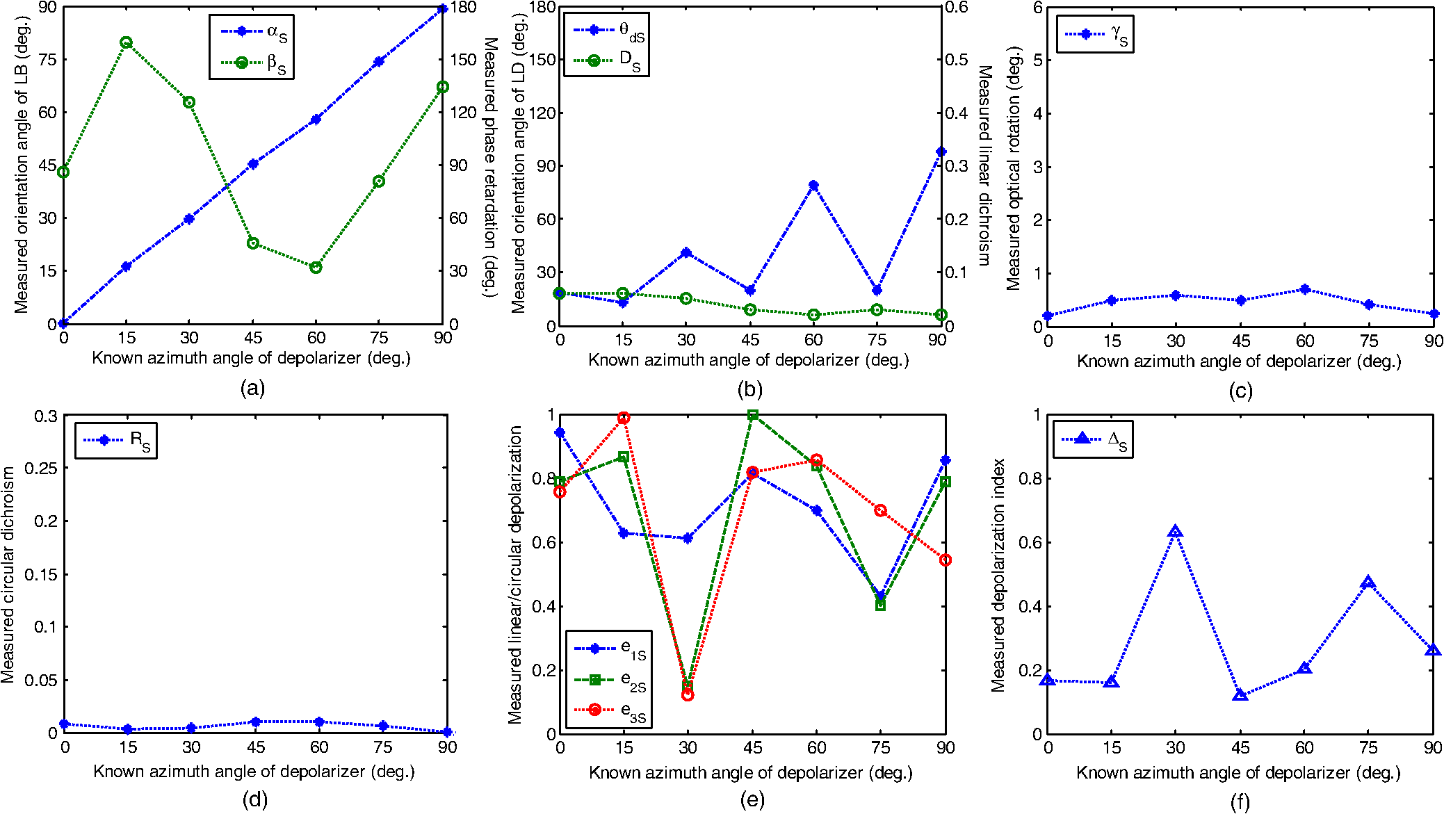
In practice, many biological samples do not possess all nine effective optical parameters. For example, collagen and muscle samples have only LB/depolarization properties, protein samples have CB/CD/depolarization properties, while diabetes samples have only CB/depolarization properties. Utilizing the input Mueller matrices provided in Refs. 23 and 25 for further investigation purposes, it was found that for samples having one or a few optical properties, the extracted parameter values were in good agreement with the input values for all six decomposition sequences. In other words, the analytical method proposed in this study provides a reliable means of extracting the effective parameters of real-world samples, regardless of the sequence in which the depolarizing Mueller matrix is decomposed.

5. Experimental Setup and Results for Measurement of Nine Effective Parameters of Anisotropic Materials

5.1.

Experimental Setup

Figure 2 presents a schematic illustration of the experimental setup used in the present study to characterize the LB, LD, CB, CD, L-Dep and C-Dep properties of turbid media. In performing the experiments, the input light was provided by a frequency-stable He-Ne laser (SL 02/2, SIOS Co.) with a central wavelength of 632.8 nm. In addition, a polarizer (GTH5M, Thorlabs Co.) and quarter-wave plate (QWP0-633-04-4-R10, CVI Co.) were used to produce four linear polarization lights (0 deg, 45 deg, 90 deg and 135 deg) and two circular polarization lights (right-handed and left-handed). Finally, a neutral density filter (NDC-100-2, ONSET Co.) and power meter detector (8842A, OPHIT Co.) were used to ensure that each of the input polarization lights had an identical intensity. (Note that for samples with no LD, the output Stokes parameters can be normalized as $S_{C} / S_{0}$ since the terms $m_{12}$ , $m_{13}$ and $m_{14}$ in Eq. (3) are nonzero. Thus, there is no need to calibrate the intensity of the input light. However, for samples with dichroism, the output Stokes parameters cannot be normalized in this way and thus the neutral density filter and power meter detector are required.)

Fig. 2

Schematic illustration of experimental measurement system.

The output Stokes parameters were computed from the intensity measurements obtained using a commercial Stokes polarimeter (PAX5710, Thorlabs Co.) at a sampling rate of 30 samples per second. A minimum of 1024 data points were obtained for each sample. Of these data points, 100 points were chosen and used to calculate the mean value of each effective parameter. It is noted that the experimental data were chosen from the average result of four to five multiple measurements.

The validity of the proposed measurement method was evaluated using three different optical samples, namely a polymer polarizer (LLC2-82-18S, OPTIMAX Co.) baked in an oven at a temperature of 150°C for 100 min; a quartz depolarizer; and a composite sample comprising a quartz depolarizer and a quarter-wave plate. The baked polarizer was chosen to evaluate the performance of the proposed measurement system in measuring the optical parameters of samples with both LB and LD properties, while the depolarizer was picked to evaluate the performance of the proposed measurement system in extracting the optical parameters of samples with depolarization properties. In addition, the composite sample was selected to evaluate the performance of the proposed measurement system in extracting the optical parameters of turbid media with both LB and depolarization properties.

5.2.

Experimental Results

5.2.1.

Baked polarizer (LB and LD properties)

Figure 3 illustrates the experimental results obtained for the LB and LD properties of the baked polarizer. The average measured values of the nine effective optical parameters of baked polarizer with different orientation angle of LD from 0 to 180 deg in increments of 30 deg are summarized. As expected, the measured values of the optical rotation angle ( $γ$ ), CD ( $R$ ), and depolarization index ( $Δ_{S}$ ) are close to zero [see Fig. 3(c) to 3(e)]. Due to the prolonged exposure of the polarizer to a high-temperature environment, the input light leaks through one of the dichroism axes. Thus, as shown in Fig. 3(b), the average value of the LD (D) is found to be 0.974. A good agreement is observed between the measured values of the LD orientation angle ( $θ_{d}$ ) and the given values. Figure 3(a) shows that the baked polarizer displays a distinct LB property; the average value of the phase retardance ( $β$ ) is found to be 16.92 deg. In addition, a good agreement is observed between the measured values of the LB orientation angle and the given values. From inspection, the standard deviations of the extracted values of $α$ , $β$ , $θ_{d}$ and D are found to be just 0.07 deg, 0.06 deg, 0.01 deg and $3.4 \times 10^{- 5}$ , respectively. In other words, the proposed analytical model enables the parameters of optical samples with both LB and LD properties to be accurately determined.

Fig. 3

Experimental results for nine effective properties of baked polarizer (BP).

5.2.2.

Depolarizer (L-Dep and C-Dep properties)

Figure 4 illustrates the experimental results obtained for the effective properties of the quartz depolarizer (DEQ-1N in ONSET Co.). The depolarizer converts the linearly polarized input beams to unpolarized beams with an orientation of 45 deg relative to the optical axis (ONSET Co.). As expected, Fig. 4(e) shows that the degrees of linear/circular depolarization fall within the range of zero to one over the considered azimuth angle range of 0 to 90 deg. Thus, the depolarization index of the depolarizer has a value between 0.2 and 0.6, as shown in Fig. 4(f). It is noted that the depolarization index has a higher value for azimuth angles of 30 deg or 75 deg. As shown in Fig. 4(a), the extracted value of the retardance varies randomly in the range of 0 to 180 deg as the azimuth angle of the depolarizer is increased. Figure 4(b) shows that the LD of the depolarizer is close to zero. Thus, the extracted value of the LD orientation angle varies randomly in the range of 0 to 180 deg as the azimuth angle of the depolarizer is increased. Finally, as expected, Fig. 4(c) and 4(d) shows that the optical rotation angle and CD of the depolarizer are both close to zero.

Fig. 4

Experimental results obtained for nine effective properties of depolarizer.

5.2.3.

Composite sample comprising depolarizer and quarter-wave plate (LB, L-Dep and C-Dep properties)

Table 4 summarizes the experimental results obtained for the effective parameters of a quarter-wave plate (QWP0-633-04-4-R10, CVI Co.), a depolarizer (DEQ-1N, ONSET Co.), and a composite sample comprising the quarter-wave plate and depolarizer given principal axis angles of 30 deg and 45 deg. This shows a good agreement exists between the LB orientation angles of the quarter-wave plate, depolarizer and composite sample for both values of the principal axis angle. The average value of LB orientation angles of the quarter-wave plate, the depolarizer, and the composite sample are found to be 30.12 deg, 29.7 deg, and 30.21 deg at 30 deg and 45.00 deg, 45.4 deg, and 44.97 deg at 45 deg at the given principal axis angle, respectively. Moreover, note that the retardance of the composite sample is equal to the sum of the depolarizer and quarter-wave plate retardance values for both given principal axis angles. For example, at a 30 deg principal axis angle, the measured value of LB of the composite sample is 216.2 deg that is equivalent to the sum of 90.24 deg of the quarter-wave plate and 125.91 deg of the depolarizer. It is the same case at 45 deg of the given principal axis angle. Notice that the optical rotation angle of the composite sample is equivalent to the sum of the optical rotation angle of the depolarizer and quarter-wave at the 30 deg and 45 deg given principal axis angle. For example, at the 30 deg given principal axis angle, the measured value of CB of the composite sample is 0.72 deg that is equivalent to the sum of 0.12 deg of the quarter-wave plate and 0.6 deg of the depolarizer; and also the same case at the 45 deg given principal axis angle. In addition, the measured average values of the linear/CD of the quarter-wave plate, depolarizer and composite sample are all close to zero. As discussed in Sec. 3.2, the proposed analytical model yields reliable results for the orientation angle of LD only for samples with a LD greater than or equal to 0.05. In the present samples, the LD is close to zero, and thus the orientation angle of LD varies randomly in the range of $0 \sim 180 \deg$ at 30 deg and at 45 deg for the given principal axis angle. Finally, it is seen that the degrees of linear/circular depolarization and the depolarization index of the composite sample are in good agreement with those of the depolarizer. The standard deviations of the extracted values of $α$ , $β$ , $θ_{d}$ , $D$ , $γ$ , and $R$ are found to be just 0.09 deg, 0.06 deg, 0.12 deg, 0.003 deg, 0.01 deg and 0.001, respectively in the composite sample of a 45-deg given principal axis angle.

Table 4

Experimental results for effective parameters of quarter-wave plate, depolarizer, and composite sample.

Degree	30 deg			45 deg
Parameters	Quarter-wave plate	Depolarizer	$Quarter - wave plate + Depolarizer$	Quarter-wave plate	Depolarizer	$Quarter - wave plate + Depolarizer$
$α$	30.12 deg	29.7 deg	30.21 deg	45.00 deg	45.4 deg	44.97 deg
$β$	90.24 deg	125.91 deg	36.2 deg ( $\approx 216.2 \deg$ )	89.97 deg	45.78 deg	134.95 deg
$θ_{d}$	160.03 deg	40.92 deg	18.25 deg	31.1 deg	19.77 deg	14.88 deg
$D$	0.005	0.05	0.06	0.01	0.03	0.05
$γ$	0.12 deg	0.6 deg	0.72 deg	0.18 deg	0.5 deg	0.7 deg
$R$	0.003	0.002	0.002	0.002	0.01	0.002
$e_{1}$	1	0.611	0.609	0.999	0.816	0.813
$e_{2}$	1	0.151	0.153	1	1	1
$e_{3}$	1	0.121	0.119	1	0.817	0.818
$Δ$	0	0.630	0.631	0	0.118	0.119

Overall, the results presented in this section demonstrate the ability of the analytical model proposed in Sec. 2 to extract the nine effective parameters of samples with linear/CB, linear/CD and linear/circular depolarization properties. The decoupling of the LB, CB, LD, CD, L-Dep and C-Dep parameters in the analytical model is beneficial in maintaining the accuracy of the experimental results. For example, even though the LD orientation angle measurements shown in Fig. 4(b) are unreliable, the accuracy of the other extracted parameters is unaffected. It is noted that if the depolarization matrix in the nine-parameter model is a unit matrix, the LD and CD formalisms given in Eqs. (11), (12), and (15) are the same as those derived in the six-parameter model given in Ref. 31. Thus, the additional demonstrations on CD property can be found in Ref. 31.

6. Experimental Results for Measurement of Nine Effective Parameters of Samples Comprising D-glucose (CB, L-Dep and C-Dep properties)

6.1.

Measurement of D-Glucose Concentration

The performance of the proposed method in measuring the optical parameters of turbid media with CB, L-Dep and C-Dep properties was evaluated using three samples containing dissolved D-glucose powder ( $C_{6} H_{12} O_{6}$ , Merck Ltd.), namely an aqueous suspension of polystyrene beads with a diameter of 5 μm, an aqueous suspension of polystyrene beads with a diameter of 9 μm, and deionized (DI) water. The polystyrene bead suspensions were purchased from Thermo Scientific Ltd. and had approximate concentrations of 0.32% solids (5 μm beads) and 0.33% solids (9 μm beads), respectively. The density of both suspended particles was equal to $1.05 g / {cm}^{3}$ , while that of the D-glucose powder was $1.54 g / {cm}^{3}$ . The various solutions (each with a volume of 2 mL) were contained in square glass containers with an external depth of 12.5 mm and an internal depth of 10 mm. In performing the experiments, the distance between the center of the sample and the detector of Stokes polarimeter was set as 23 mm in every case.

Figure 5 presents the experimental results obtained for the nine effective properties of the sample comprising 5-μm diameter polystyrene beads and dissolved D-glucose powder. Note that the extracted parameter values are presented for D-glucose concentrations ranging from 0 through 1 M (Molar) in increments of 0.1 M. As shown in Fig. 5(c), the measured value of the optical rotation angle increases approximately linearly with an increasing D-glucose concentration over the considered range of 0 through 1 M. From inspection, the sensitivity of the D-glucose measurement is estimated to be $1.71 degree / M$ . The standard deviation of the optical rotation angle is found to be 0.05 deg. It is noted that the standard deviation is the maximum distance between the mean value and 100 chosen data points of optical rotation angle. The experimental data were chosen from the average result of multiple measurements. Figure 5(a) shows that the measured value of the LB orientation angle increases approximately linearly with an increasing D-glucose concentration. Meanwhile, the average value of the phase retardance is found to be 6.12 deg. Note that if the distance between the sample and the detector was specified as 65 mm for 5-μm polystyrene bead sample (Sec. 6.2), the measured values of the LB are close to zero. As in the analytical models presented in Refs. 31 32.–33, the analytical model proposed in this study yields reliable results for the LD orientation angle only for samples with a LD greater than or equal to 0.05. Figure 5(b) shows that the LD of the D-glucose sample is close to zero. Thus, the extracted values of the LD orientation angle vary randomly as the D-glucose concentration is increased. Figure 5(d) shows that the CD of the D-glucose solution is also close to zero. Figure 5(e) shows that the degrees of linear/circular depolarization all increase approximately linearly with an increasing D-glucose concentration. Moreover, as shown in Fig. 5(f), the depolarization index reduces progressively from 0.351 to 0.252 as the D-glucose concentration is increased over the considered range.

Fig. 5

Experimental results for effective properties of polystyrene microsphere suspension (5 μm) containing dissolved D-glucose powder.

Figure 6 presents the experimental results for the nine effective properties of the sample comprising 9-μm diameter polystyrene beads and dissolved D-glucose powder. It is seen in Fig. 6(c) that the optical rotation angle increases in a near linearly manner with an increasing D-glucose concentration over the considered range of 0 to 1 M. From inspection, the sensitivity of the D-glucose measurement is estimated to be $1.76 \deg / M$ , while the standard deviation of the optical rotation angle is found to be 0.04 deg. Figure 6(a) and 6(b) shows that the sample’s phase retardance and LD are both close to zero. Thus, the extracted values of the LB and LD orientation angles vary randomly as the D-glucose concentration is increased. Again, note that if the distance between the sample and the detector was specified as 15 mm for 9-μm polystyrene bead sample (Sec. 6.2), the measured values of the LB are closer to zero ( $< 0.2 \deg$ ). Figure 6(d) shows that the CD of the D-glucose solution is also close to zero. Meanwhile, Fig. 6(e) shows that the degrees of linear/circular depolarization are close to one, particularly at higher values of the D-glucose concentration. Thus, as shown in Fig. 6(f), the depolarization index has a value close to zero and reduces progressively from 0.042 to 0.023 as the D-glucose concentration is increased. As stated earlier, both polystyrene beads have the same density of $1.05 g / {cm}^{3}$ . In other words, given a constant sample volume (2 mL), the number of 9-μm diameter beads is much less than the number of 5-μm diameter beads and the numbers of beads are inversely proportional to the cubes of their radii. Thus, it is found that the scattering cross-section of the sphere particle is inversely proportional to its radius. So in comparing Figs. 5(f) and 6(f), the depolarization index of the sample containing 9-μm diameter beads is lower than that of the sample containing 5-μm diameter beads. Moreover, in the experimental results, degree of polarization (DOP) of 9-μm diameter beads sample is very high (97%) while DOP of the 5-μm diameter beads sample is smaller (around 65%).

Fig. 6

Experimental results for effective properties of polystyrene microsphere suspension (9 μm) containing dissolved D-glucose powder.

Once again, the results presented in Figs. 5 and 6 confirm the importance of decoupling the LB, CB, LD, CD, L-Dep and C-Dep parameters in the analytical model. For example, even though the extracted values of the LB and LD orientation angles in Figs. 5 and 6 are unreliable, the ability of the model to extract the remaining parameter values is unaffected.

Figure 7(a) illustrates the experimental results obtained for the optical rotation angles ( $γ$ ) of the three D-glucose samples (i.e., 5-μm beads, 9-μm beads and DI water). This shows that the slopes of the optical rotation angle of three samples in regards to the concentration of the D-glucose solution are the same. In other words, the sensitivity of the optical rotation angle to the D-glucose concentration is equivalent for all three samples. However, the optical rotation angles of the three samples given a D-glucose concentration of 0 M are different. Specifically, the optical rotation angles of the pure DI sample are significantly higher than that of the two samples containing polystyrene beads. Moreover, the optical rotation angles of the sample containing 9-μm polystyrene beads are remarkably higher than that of the sample containing 5-μm polystyrene beads. Figure 7(b) shows a good agreement is observed among the optical rotation angles of three samples after calibration. As described in the following subsection, a calibration procedure is proposed to render the extracted optical rotation angle of the D-glucose insensitive to the suspension medium, as shown in Fig. 7(b).

Fig. 7

Variation of optical rotation angle with D-glucose concentration: (a) before calibration and (b) after calibration.

6.2.

Calibration of Optical Rotation Angle in Accordance with Distance between Sample and Detector

In experimental polarimetry configurations, such as that shown in Fig. 2, the extracted value of the optical rotation angle of particle suspensions containing D-glucose varies in accordance with the distance between the sample and the detector.²³ Figure 8(a) and 8(b) shows the experimental results obtained for the optical rotation angles of the present suspended microsphere samples with and without D-glucose, respectively, given various distances between the center of the sample and the detector of Stokes polarimeter. Figure 8(a) shows that given a D-glucose concentration of 0 M, the maximum values of the optical rotation angle are obtained at a distance of 65 mm for the 5-μm bead sample and 15 mm for the 9-μm bead sample. Figure 8(b) shows that given a D-glucose concentration of 0.6 M, the maximum optical rotation angles of the two samples are again obtained at distances of 65 mm and 15 mm, respectively. Note that the extracted value of the LB of particle suspensions containing D-glucose also varies in accordance with the distance between the sample and the detector. Interestingly, the extracted values of LB of both two bead samples are close to zero when the maximal value of the optical rotation angle is chosen in calibration. This means if the distance between the sample and the detector was specified as 65 mm for the 5-μm polystyrene bead sample and as 15 mm for the 9-μm polystyrene bead sample, the measured values of the LB are close to zero ( $< 0.2 \deg$ ). The depolarization values do not change much ( $< 0.02$ ) in accordance with the distance between the sample and the detector. Accordingly, in performing the remaining experiments, the distance between the sample and the detector was specified as 65 mm for the 5-μm polystyrene bead sample and 15 mm for the 9-μm polystyrene bead sample. Figure 9 shows the variation of the optical rotation angle of the two polystyrene bead/glucose samples with the D-glucose concentration over the range of 0 to 0.6 M. The results confirm that the optical rotation angle of both samples–given a D-glucose concentration of 0 M—is equal to zero following the calibration process. From inspection, the sensitivity of the D-glucose measurement is estimated to be $1.73 degree / M$ . In other words, the ability of the proposed (calibrated) method to extract the properties of turbid samples with CB is confirmed.

Fig. 8

Variation of optical rotation angles of polystyrene microsphere solutions with sample-to-detector distance given: (a) 0 M D-glucose concentration, and (b) 0.6 M D-glucose concentration.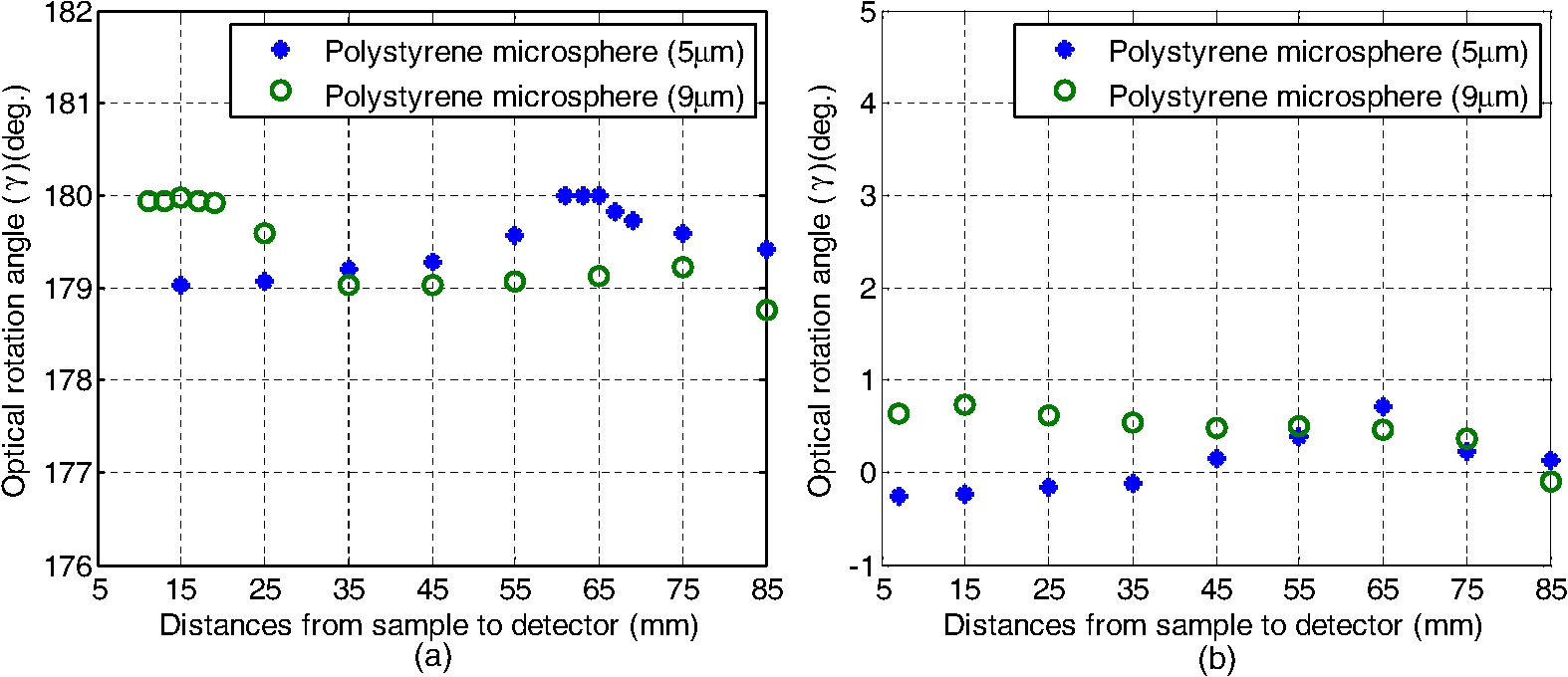

Fig. 9

Variation of optical rotation angle of D-glucose solutions containing polystyrene microspheres with D-glucose concentration following sample-to-detector calibration process.

In summary, the experimental results confirm that the decoupled nature of the analytical model improves accuracy and the ability to extract the parameters of optical samples with only one or many properties of LB/CB, LD/CD, L-Dep/C-Dep. Moreover, the decoupling of the LB, CB, LD, CD, L-Dep and C-Dep parameters in the analytical model is beneficial in maintaining the accuracy of the experimental results. The method is also proposed for calibrating the optical rotation angle of a polystyrene microsphere suspension containing dissolved D-glucose powder in accordance with the distance between the sample and the detector. For the sample with unknown bead size, a calibration will be made for finding the maximal value of the optical rotation angle in accordance with the distance between the sample and the detector.

7. Conclusions and Discussions

This study proposed a decoupled analytical technique based on Stokes polarimetry and the Mueller matrix method for extracting the nine effective LB, LD, CB, CD, L-Dep (L-Dep), and circular depolarization (C-Dep) properties of turbid optical samples. The experimental results show that the decoupled nature of the analytical model localizes the effects of measurement errors and enables the properties of pure LB, LD, CB, CD, L-Dep or C-Dep samples to be extracted without the need for any form of compensation process or pretreatment. A method has been proposed for calibrating the extracted value of the optical rotation angle for turbid samples comprising D-glucose dissolved within a polystyrene microsphere solution in accordance with the distance between the sample and the detector of Stokes polarimeter. The results demonstrate that the calibrated analytical model enables the properties of turbid samples with CB to be successfully determined. In general, the results presented in this study show that the proposed method has the potential for such applications as collagen and muscle structure characterization (based on LB/Depolarization measurements), protein structure characterization (based on CB/CD/Depolarization measurements) or diabetes detection (based on CB/Depolarization measurements).

Acknowledgments

The authors gratefully acknowledge the financial support provided for this study by the National Science Council of Taiwan under Grant No. NSC99-2221-E-006-034-MY3.

References

1.

P. R. Bargoet al., “In vivo determination of optical properties of normal and tumor tissue with white light reflectance and an empirical light transport model during endoscopy,” J. Biomed. Opt., 10 (3), 034018 (2005). http://dx.doi.org/10.1117/1.1921907 JBOPFO 1083-3668 Google Scholar

2.

T. MoffittY. C. ChenS. A. Prahl, “Preparation and characterization of polyurethane optical phantoms,” J. Biomed. Opt., 11 (4), 041103 (2006). http://dx.doi.org/10.1117/1.2240972 JBOPFO 1083-3668 Google Scholar

3.

J. W. Pickeringet al., “Double-integrating-sphere system for measuring the optical properties of tissue,” Appl. Opt., 32 (4), 399 –410 (1993). http://dx.doi.org/10.1364/AO.32.000399 APOPAI 0003-6935 Google Scholar

4.

A. A. OraevskyS. L. JacquesF. K. Tittel, “Measurement of tissue optical properties by time-resolved detection of laser-induced transient stress,” Appl. Opt., 36 (1), 402 –415 (1997). http://dx.doi.org/10.1364/AO.36.000402 APOPAI 0003-6935 Google Scholar

5.

S. J. MatcherM. CopeD. T. Delpy, “In vivo measurements of the wavelength dependence of tissue-scattering coefficients between 760 and 900 nm measured with time-resolved spectroscopy,” Appl. Opt., 36 (1), 386 –396 (1997). http://dx.doi.org/10.1364/AO.36.000386 APOPAI 0003-6935 Google Scholar

6.

G. Palet al., “Time-resolved optical tomography using short-pulse laser for tumor detection,” Appl. Opt., 45 (24), 6270 –6282 (2006). http://dx.doi.org/10.1364/AO.45.006270 APOPAI 0003-6935 Google Scholar

7.

D. Continiet al., “Multi-channel time-resolved system for functional near infrared spectroscopy,” Opt. Express, 14 (12), 5418 –5432 (2006). http://dx.doi.org/10.1364/OE.14.005418 OPEXFF 1094-4087 Google Scholar

8.

S. Fantiniet al., “Frequency-domain multichannel optical detector for noninvasive tissue spectroscopy and oximetry,” Opt. Eng., 34 (1), 32 –42 (1995). http://dx.doi.org/10.1117/12.183988 OPEGAR 0091-3286 Google Scholar

9.

G. Alexandrakiset al., “Determination of the optical properties of two-layer turbid media by use of a frequency-domain hybrid Monte Carlo diffusion model,” Appl. Opt., 40 (22), 3810 –3821 (2001). http://dx.doi.org/10.1364/AO.40.003810 APOPAI 0003-6935 Google Scholar

10.

N. Shahet al., “Spatial variations in optical and physiological properties of healthy breast tissue,” J. Biomed. Opt., 9 (3), 534 –540 (2004). http://dx.doi.org/10.1117/1.1695560 JBOPFO 1083-3668 Google Scholar

11.

S. Yehet al., “Near-infrared thermo-optical response of the localized reﬂectance of intact diabetic and nondiabetic human skin,” J. Biomed. Opt., 8 (3), 534 –544 (2003). http://dx.doi.org/10.1117/1.1578641 JBOPFO 1083-3668 Google Scholar

12.

A. DimofteJ. FinlayT. Zhu, “A method for determination of the absorption and scattering properties interstitially in turbid media,” Phys. Med. Biol., 50 (10), 2291 –2311 (2005). http://dx.doi.org/10.1088/0031-9155/50/10/008 PHMBA7 0031-9155 Google Scholar

13.

R. O. Esenalievet al., “Continuous noninvasive monitoring of total hemoglobin concentration by an optoacoustic technique,” Appl. Opt., 43 (17), 3401 –3407 (2004). http://dx.doi.org/10.1364/AO.43.003401 APOPAI 0003-6935 Google Scholar

14.

C. L. DarlingG. D. HuynhD. Fried, “Light scattering properties of natural and artiﬁcially demineralized dental enamel at 1310 nm,” J. Biomed. Opt., 11 (3), 034023 (2006). http://dx.doi.org/10.1117/1.2204603 JBOPFO 1083-3668 Google Scholar

15.

B. D. Cameronet al., “Measurement and calculation of the two-dimensional backscattering Mueller matrix of a turbid medium,” Opt. Lett., 23 (7), 485 –487 (1998). http://dx.doi.org/10.1364/OL.23.000485 OPLEDP 0146-9592 Google Scholar

16.

G. L. LiuY. LiB. D. Cameron, “Polarization-based optical imaging and processing techniques with application to the cancer diagnostics,” Proc. SPIE, 4617 208 –220 (2002). http://dx.doi.org/10.1117/12.472527 PSISDG 0277-786X Google Scholar

17.

B. D. CameronY. LiA. Nezhuvingal, “Determination of optical scattering properties in turbid media using Mueller matrix imaging,” J. Biomed. Opt., 11 (5), 054031 (2006). http://dx.doi.org/10.1117/1.2363347 JBOPFO 1083-3668 Google Scholar

18.

Y. Denget al., “Characterization of backscattering Mueller matrix patterns of highly scattering media with triple scattering assumption,” Opt. Express, 15 (15), 9672 –9680 (2007). http://dx.doi.org/10.1364/OE.15.009672 OPEXFF 1094-4087 Google Scholar

19.

Y. Denget al., “Numerical study of the effects of scatterer sizes and distributions on multiple backscattered intensity patterns of polarized light,” Opt. Lett., 33 (1), 77 –79 (2008). http://dx.doi.org/10.1364/OL.33.000077 OPLEDP 0146-9592 Google Scholar

20.

X. WangG. YaoL. V. Wang, “Monte Carlo model and single-scattering approximation of the propagation of polarized light in turbid media containing glucose,” Appl. Opt., 41 (4), 792 –801 (2002). http://dx.doi.org/10.1364/AO.41.000792 APOPAI 0003-6935 Google Scholar

21.

X. WangL. V. Wang, “Propagation of polarized light in birefringent turbid media: a Monte Carlo study,” J. Biomed. Opt., 7 (3), 279 –290 (2002). http://dx.doi.org/10.1117/1.1483315 JBOPFO 1083-3668 Google Scholar

22.

N. Ghoshet al., “Mueller matrix decomposition for polarized light assessment of biological tissues,” J. Biophotonics, 2 (3), 145 –156 (2009). http://dx.doi.org/10.1002/jbio.v2:3 JBOIBX 1864-063X Google Scholar

23.

N. GhoshM. F. G. WoodI. A. Vitkin, “Polarimetry in turbid, birefringent, optically active media: A Monte Carlo study of Mueller matrix decomposition in the backscattering geometry,” J. Appl. Phys., 105 (10), 102023 (2009). http://dx.doi.org/10.1063/1.3116129 JAPIAU 0021-8979 Google Scholar

24.

X. Guoet al., “Depolarization of light in turbid media: a scattering event resolved Monte Carlo study,” Appl. Opt., 49 (2), 153 –162 (2010). http://dx.doi.org/10.1364/AO.49.000153 APOPAI 0003-6935 Google Scholar

25.

N. GhoshI. A. Vitkin, “Tissue polarimetry: concepts, challenges, applications, and outlook,” J. Biomed. Opt., 16 (11), 110801 (2011). http://dx.doi.org/10.1117/1.3652896 JBOPFO 1083-3668 Google Scholar

26.

S. Y. LuR. A. Chipman, “Interpretation of Mueller matrices based on polar decomposition,” J. Opt. Soc. Am. A, 13 (5), 1106 –1113 (1996). http://dx.doi.org/10.1364/JOSAA.13.001106 0740-3232 Google Scholar

27.

R. M. A. Azzam, “Propagation of partially polarized light through anisotropic media with or without depolarization: A differential

4 \times 4

matrix calculus,” J. Opt. Soc. Am., 68 (12), 1756 –1767 (1978). http://dx.doi.org/10.1364/JOSA.68.001756 JOSAAH 0030-3941 Google Scholar

28.

R. Ossikovski, “Differential matrix formalism for depolarizing anisotropic media,” Opt. Lett., 36 (12), 2330 –2332 (2011). http://dx.doi.org/10.1364/OL.36.002330 OPLEDP 0146-9592 Google Scholar

29.

N. Ortega-QuijanoJ. L. Arce-Diego, “Depolarizing differential Mueller matrices,” Opt. Lett., 36 (13), 2429 –2431 (2011). http://dx.doi.org/10.1364/OL.36.002429 OPLEDP 0146-9592 Google Scholar

30.

N. Ortega-QuijanoJ. L. Arce-Diego, “Mueller matrix differential decomposition,” Opt. Lett., 36 (10), 1942 –1944 (2011). http://dx.doi.org/10.1364/OL.36.001942 OPLEDP 0146-9592 Google Scholar

31.

T. T. H. PhamY. L. Lo, “Extraction of effective parameters of anisotropic optical materials using decoupled analytical method,” J. Biomed. Opt., 17 (2), 25006 (2012). http://dx.doi.org/10.1117/1.JBO.17.2.025006 JBOPFO 1083-3668 Google Scholar

32.

P. C. Chenet al., “Measurement of linear birefringence and diattenuation properties of optical samples using polarimeter and Stokes parameters,” Opt. Express, 17 (18), 15860 –15884 (2009). http://dx.doi.org/10.1364/OE.17.015860 OPEXFF 1094-4087 Google Scholar

33.

Y. L. LoT. T. H. PhamP. C. Chen, “Characterization on five effective parameters of anisotropic optical material using Stokes parameters-Demonstration by a fiber-type polarimeter,” Opt. Express, 18 (9), 9133 –9150 (2010). http://dx.doi.org/10.1364/OE.18.009133 OPEXFF 1094-4087 Google Scholar

34.

B. J. DeBooJ. M. SasianR. A. Chipman, “Depolarization of diffusely reflecting man-made objects,” Appl. Opt., 44 (26), 5434 –5445 (2005). http://dx.doi.org/10.1364/AO.44.005434 APOPAI 0003-6935 Google Scholar

35.

J. J. GilE. Bernabeu, “Depolarization and polarization indices of an optical system,” Opt. Acta., 33 (2), 185 –189 (1986). http://dx.doi.org/10.1080/713821924 OPACAT 0030-3909 Google Scholar

36.

J. SchellmanH. P. Jensen, “Optical spectroscopy of oriented molecules,” Chem. Rev., 87 (6), 1359 –1399 (1987). http://dx.doi.org/10.1021/cr00082a004 0009-2665 Google Scholar

37.

O. ArteagaA. Canillas, “Analytic inversion of the Mueller-Jones polarization matrices for homogeneous media,” Opt. Lett., 35 (4), 559 –561 (2010). http://dx.doi.org/10.1364/OL.35.000559 OPLEDP 0146-9592 Google Scholar

38.

J. MorioF. Goudail, “Inﬂuence of the order of diattenuator, retarder and polarizer in polar decomposition of Mueller matrices,” Opt. Lett., 29 (19), 2234 –2236 (2004). http://dx.doi.org/10.1364/OL.29.002234 OPLEDP 0146-9592 Google Scholar

39.

T. T. H. PhamY. L. LoP. C. Chen, “Design of polarization-insensitive optical fiber probe based on effective optical parameters,” J. Lightwave. Tech., 29 (8), 1127 –1135 (2011). http://dx.doi.org/10.1109/JLT.2011.2123870 JLTEDG 0733-8724 Google Scholar

Citation Download Citation

Thi-Thu-Hien Pham and Yu-Lung Lo "Extraction of effective parameters of turbid media utilizing the Mueller matrix approach: study of glucose sensing," Journal of Biomedical Optics 17(9), 097002 (6 September 2012). https://doi.org/10.1117/1.JBO.17.9.097002

Published: 6 September 2012

Access the abstract

JOURNAL ARTICLE
15 PAGES

DOWNLOAD PAPER SAVE TO MY LIBRARY

GET CITATION

CITATIONS

Cited by 36 scholarly publications and 2 patents.

Explore citations on Lens.org

RIGHTS & PERMISSIONS

Get copyright permission Get copyright permission on Copyright Marketplace

KEYWORDS

Dichroic materials

Statistical analysis

Statistical modeling

Sensors

Error analysis

Calibration

Composites

1.

Introduction

2.

Proposed Analytical Model for Extracting Nine Effective Optical Parameters of Turbid Media

Eq. (1)

Eq. (2)

Eq. (3)

Fig. 1

Table 1

Eq. (4)

Eq. (5)

Eq. (6)

Eq. (7)

Eq. (8)

Eq. (9)

Eq. (10)

Eq. (11)

Eq. (12)

Eq. (13)

Eq. (14)

Eq. (15)

Eq. (16)

Eq. (17)

Eq. (18)

Eq. (19)

Eq. (20)

Eq. (21)

Eq. (22)

Eq. (23)

Eq. (24)

Eq. (25)

Eq. (26)

Eq. (27)

Eq. (28)

Eq. (29)

Eq. (30)

Eq. (31)

Eq. (32)

Eq. (33)

Eq. (34)

Eq. (35)

Eq. (36)

Eq. (37)

Eq. (38)

Eq. (39)

Eq. (40)

3.

Analytical Simulations and Error Analysis

3.1.

Analytical Simulations

3.2.

Error Analysis of Proposed Measurement Methodology

3.3.

Comparison of Results Extracted using Analytical Model and those Presented in the Literature

Table 2

4.

Effect of [MΔ], [MR] and [MD] Decomposition Order

Eq. (41)

Table 3

5.

Experimental Setup and Results for Measurement of Nine Effective Parameters of Anisotropic Materials

5.1.

Experimental Setup

Fig. 2

5.2.

Experimental Results

5.2.1.

Baked polarizer (LB and LD properties)

Fig. 3

5.2.2.

Depolarizer (L-Dep and C-Dep properties)

Fig. 4

5.2.3.

Composite sample comprising depolarizer and quarter-wave plate (LB, L-Dep and C-Dep properties)

Table 4

6.

Experimental Results for Measurement of Nine Effective Parameters of Samples Comprising D-glucose (CB, L-Dep and C-Dep properties)

6.1.

Measurement of D-Glucose Concentration

Fig. 5

Effect of $[M_{Δ}]$ , $[M_{R}]$ and $[M_{D}]$ Decomposition Order