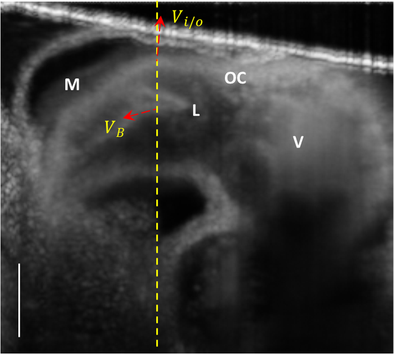
1.

Introduction

Optical coherence tomography (OCT) is a powerful, noninvasive imaging technique, capable of imaging highly scattering biological tissue, either in vitro or in vivo, with high temporal ($\sim \mathrm{\mu s}$ range) and spatial ($\sim \mathrm{\mu m}$) resolutions.^1–6 Due to the high scattering nature of biological tissues, the imaging depth for OCT is, however, limited to 2.0 mm. Nevertheless, these attributes make OCT uniquely suited for the study of embryonic heart development.^4,7–14 because of the relatively small size of the heart at early developmental stages. OCT has been used in a number of embryonic models, such as Rana pipiens tadpole,¹⁵ Xenopus laevis,¹⁶ zebrafish,¹⁷ chick,^9,18 and mouse.^19,20 Briefly, OCT imaging of the embryonic heart can be classified into two categories: structural imaging and functional imaging.

In an embryonic chick heart, blood flow begins at early developmental stages. At the Hamburger-Hamilton (HH) stage 18, the heart pumps blood via a peristaltic-like periodic contraction motion,²¹ and the heart rate is about 2.2 to 2.4 beats per second.²² To image the morphological dynamics of the beating heart, OCT has evolved from two-dimensional (2-D) cross sectional imaging^9,15,16 to three-dimensional (3-D)^18–20 and even four-dimensional (4-D) (time-lapse 3-D) volumetric imaging.^4,13,23 However, real-time volumetric imaging is still a big challenge because of the limited imaging speed even with the current state-of-the-art OCT system. To mitigate the limitations of OCT imaging speed, high frame rate (B-scan) is often used to resolve the fast dynamic events of the beating heart. To realize the dynamic 3-D imaging, gating technology is proposed to reconstruct the time-lapse 3-D images from the MB-mode frames (repeated B-scan at one spatial position) acquired at sequential spatial cross-sections via various synchronization techniques; for example, prospective-gating^24,25 and retrospective-gating.^4,13 The gated imaging increases the temporal resolution; however, it may lose information about the nonperiodic events during the heart beat because it is based on the periodicity of the cardiac beating. With the current improvement of swept laser source—for example, buffered Fourier domain mode locked laser—the OCT system (i.e. swept source OCT [SSOCT]) has been demonstrated to have $>100\text{-}\text{kHz}$ line scan rate, providing volumetric imaging of 10 volumes per second (70 frames with each frame consisting of 150 A-lines).²³ Although such ultrafast swept laser source is desirable to study the morphological dynamics, the ultrafast swept source OCT is not currently commercially available. Moreover, although several methods have been proposed for improving the phase stability of swept source, and great improvement has been achieved,²⁶ the relatively poor performance of typical SSOCT system in phase stability still limits its application in the study of hemodynamics compared with the OCT system that uses a broadband superluminescent light source, i.e., spectral domain OCT (SDOCT). A primary advantage of the SDOCT over the SSOCT is its stable phase signal, offering the capability to image the tissue motion and blood flow using the Doppler principle.^27,28 However, the imaging speed of SDOCT is mainly determined by the availability of high-speed camera used in the spectrometer to detect the spectrograms formed between the reference and sample lights.

At 1310-nm wavelength band, the fastest camera available so far is 92 kHz, which determines the achievable imaging speed for SDOCT.^29–31 In order to improve the imaging speed beyond this limit, An et al. recently proposed a method that employs two identical spectrometers that are externally triggered by precisely controlled trigger-signals.³² Equipped with an InGaAs line-scan camera operating at 92-kHz line scan rate in each of the spectrometers, this method has enabled SDOCT to operate at 184 kHz. With this imaging speed, it is foreseeable that such system would not only provide a competitive temporal resolution in the study of morphological dynamics, but also facilitates the study of hemodynamics in the fast beating embryonic heart because it offers a capability to resolve a flow speed of $\sim 43.95\mathrm{mm}/\mathrm{s}$ within living tissue.

During the cardiac cycle, the developing cardiac wall (composed of myocardium, cardiac jelly, and endocardium) and the flowing blood constantly interact with each other, which determines the biomechanical environment that in turn regulates cardiac development. A dilemma exits, however, when studying the dynamic interaction between the cardiac wall and the blood flow because the motion of cardiac wall is relatively slow compared to the fast flow of blood. The slow motion of the cardiac wall requires the OCT system operating at a slower imaging speed, whereas the fast motion of blood demands a faster imaging speed. Previously, considerable efforts have been paid to the measurements of the blood flow velocity, from which biomechanical parameters, such as shear rate¹¹ and shear stress,^5,33 were calculated. In order to better understand the dynamic wall motion, Li et al. proposed a method to directly assess the in vivo radial strain rate (SR) of the myocardial wall in the early embryonic chick heart by the use of phase-resolved tissue Doppler OCT technology.³⁴ In that study, the velocity of tissue (myocardium) was obtained by calculating the phase shift $\mathrm{\Delta }\phi$ between adjacent A-lines in the same B-frame. A drawback of this approach is that the time interval $\tau$ between adjacent A-lines is extremely short (on the scale of microseconds), making the measurement of the slow tissue motion prone to system phase noise. To improve the system sensitivity to the slow tissue motion, one has to increase the time-interval $\tau$ for the calculation of the tissue velocity $V$ while the system is still capable of measuring the velocity of the fast blood flow.

In this pilot study, we report the use of 184-kHz SDOCT system to provide simultaneous quantification of blood flow and cardiac wall SR in the outflow tract (OFT) of the embryonic chick heart. The ultrafast imaging speed provides us with the ability to image the beating heart at a frame rate of 560 frames per second (fps). We use the phase-shift between adjacent B-scans to quantify the slow wall motion, while the imaging speed of the system is not sacrificed to measure the velocity of the fast blood flow that is assessed by the phase shift between adjacent A-lines within a B-scan. We present the results to demonstrate the feasibility of such approach to simultaneously measure the pulsatile blood flow and the myocardial wall motion, offering an opportunity to study the dynamic interaction between them during cardiac development.

2.

Material and Methods

2.2.

OCT System Setup

A schematic diagram of the ultrafast dual-camera SDOCT system used in this study is shown in Fig. 1, in which a broadband superluminescent diode (SLD) with a central wavelength of 1310 nm and a spectral bandwidth of 60 nm was used as the low coherence light source, theoretically providing a $\sim 12\text{-}\mathrm{\mu m}$ axial resolution in air. The emitted radiation from the SLD was first split into two portions by a fiber-optical coupler with a $10/90$ coupling ratio. These two light portions were then directed to the reference arm and the sample arm via two broadband optical circulators, respectively. In the sample arm, the light was focused onto the sample by an objective lens (focal length is $\sim 50\mathrm{mm}$), yielding a $\sim 16\text{-}\mathrm{\mu m}$ lateral resolution. The lights backscattered from the sample and reflected from the reference mirror were routed back to the circulators and then recombined by a $2\times 2$ fiber optical coupler with a $50/50$ coupling ratio. Thereafter, the interference signal was equally split into two home-built spectrometers with identical imaging performance. Each spectrometer was equipped with a state-of-the-art 92 KHz InGaAs line scan camera (SU1024LDH2, Goodrich Ltd.), which had a designed spectral resolution of $\sim 0.14\mathrm{nm}$ giving a measured imaging depth of $\sim 3.0\mathrm{mm}$ in air. The spectrometer had $\sim 102\mathrm{dB}$ sensitivity around zero-delay line and $\sim 95\mathrm{dB}$ at 1.5-mm imaging-depth position. The two spectrometers worked together by external trigger signals [Trigger 2(a) and 2(b)], providing a $\sim 184\text{-}\mathrm{KHz}$ A-line scan rate.³²

Fig. 1

Schematic of ultrafast dual-camera SDOCT system. OC: optical coupler; CIR: circulator; PC: polarization control; CL: collimating lens; FL: focusing lens; M: mirror; GV: galvanometer; OL: objective lens; DG: diffraction grating. Trigger 1: to synchronize the OCT scanning; Trigger 2a and 2b: to synchronize the data acquisition of the dual camera.

During imaging, the probe beam was scanned in the $X$-direction by a GV-X scanner driven with a saw-tooth waveform. About 256 axial A-scans were acquired to form a B-frame spatially covering $\sim 1.1\mathrm{mm}$ on the chick embryo heart that provided a $\sim 75\%$ spatial correlation between the adjacent A-lines to ensure the measurement of blood flow velocity by the use of conventional phase-resolved Doppler OCT. This arrangement of scanning also afforded a B-frame rate of 560 fps that gave us an opportunity to measure the slow wall motion by the use of the phase shift between adjacent B-scans. For each experiment, 1000 repeated B-frames were acquired, i.e. MB-mode scan, temporally covering $\sim 3$ to 4 cardiac periods of the beating heart.

2.3.

Image Analysis

The radial SR and the blood flow velocity were quantified from the captured MB mode datasets. The radial SR, ${\epsilon }^{\prime }$, is defined as the speed at which the myocardial wall thickens and thins over the cardiac cycles,^42,43 which can be evaluated by calculating the velocity gradient of the myocardial wall in the radial direction.^34,42,43 However, the velocity vector of the myocardial wall motion is inherently 3-D, which can be decomposed into three components: radial, longitudinal, and circumferential. In this study, we focused on the deformation along the central A-line [the A-line that crosses the center of OFT cross-section, please refer to the dashed line in Fig. 2(b)] so that the circumferential deformation can be neglected.

Fig. 2

Extraction of myocardial wall boundary positions from the OCT images of embryonic chick heart OFT. (a) Typical OFT longitudinal section, and (b) OFT cross-section; (c) M-mode structural image along the vertical dashed line in (b) in which the boundary of myocardial wall is indicated by the solid curves; (d) relative depth positions of the myocardial wall boundary; (e) thickness variation of the myocardial wall over $\sim 1.7\sec$ period. M: myocardium; CJ: cardiac jelly; B: blood; V: ventricle; OC: outflow cushion (endocardial cushions). The $\text{vertical scale bar}=200\mathrm{\mu m}$; the $\text{horizontal bar}=0.1\mathrm{s}$.

Because of the linear velocity distribution of the myocardial wall in the radial direction, the radial SR ${\epsilon }^{\prime }$ can be expressed by Ref. 34:

Eq. (1)

$${\epsilon }^{\prime }(t)=\frac{V_{\mathrm{ri}}(t)-V_{\mathrm{ro}}(t)}{L(t)},$$

where $L(t)$ is the instantaneous thickness of the myocardial wall. $V_{\mathrm{ri}}(t)$ and $V_{\mathrm{ro}}(t)$ are, respectively, the radial velocity of the inner and outer boundaries of the myocardial wall along the central A-line at time $t$. To facilitate the discussion, Fig. 3 shows a schematic drawing of the relationship between OCT probe beam, myocardial wall motion and blood flow direction within lumen. As shown in Fig. 3(a), the Doppler velocity $V_i(t)$ and $V_o(t)$ measured by the OCT system can be considered as the sum of the radial component and the longitudinal component:

Eq. (2)

$$V_i(t)=V_{\mathrm{ri}}(t)\cos ({\alpha }_M)+V_{\mathrm{li}}(t)\sin ({\alpha }_M)V_o(t)=V_{\mathrm{ro}}(t)\cos ({\alpha }_M)+V_{\mathrm{lo}}(t)\sin ({\alpha }_M),$$

where $V_{\mathrm{li}}(t)$ and $V_{\mathrm{lo}}(t)$ are, respectively, the longitudinal velocity of the inner and outer boundaries of the myocardial wall along the central A-line at time $t$. ${\alpha }_M$ is the angle between the radial velocity direction and the probe beam. In this study, it was assumed that the angle ${\alpha }_M$ is small enough so that $\sin ({\alpha }_M)\approx 0$, which can be met by carefully adjusting the angle during experiments. Substituting $L(t)=(z_i(t)-z_o(t))\cos ({\alpha }_M)$ and Eq. (2) in Eq. (1) allows ${\epsilon }^{\prime }(t)$ to be rewritten as:

Eq. (3)

$${\epsilon }^{\prime }(t)=\frac{V_i(t)-V_o(t)}{z_i(t)-z_o(t)}\times \frac{1}{{\cos }^2({\alpha }_M)}.$$

where $z_i(t)$ and $z_o(t)$ are the depth position of the inner and outer boundary measured from the OCT image. From the phase-resolved Doppler OCT, the Doppler velocity $V_i(t)$ and $V_o(t)$ can be evaluated from the captured MB-mode OCT datasets:

Eq. (4)

$$V_{\frac{i}{o}(t)}=\frac{\mathrm{\Delta }{\phi }_{\frac{i}{o}}(t){\lambda }_0}{4\pi nT},$$

where $\mathrm{\Delta }{\phi }_i(t)$ and $\mathrm{\Delta }{\phi }_o(t)$ are, respectively, the phase shift of the inner and outer boundaries of the myocardial wall along the central A-line at time $t$; ${\lambda }_0=1310\mathrm{nm}$ is the central wavelength of the light source; $n$ is the refractive index of the bio-tissue which is typically 1.38; $T$ is the time interval between the adjacent B-scans used for the phase shift $\mathrm{\Delta }\phi (t)$ calculation (in this case $T=1.78\mathrm{ms}$).

Fig. 3

Schematic diagram describing the relationships between the OCT probe beam, the moving myocardial wall and the blood flow within lumen: (a) for the case when evaluating the myocardial wall motion; and (b) for the case when evaluating the blood flow. $L$ is the thickness of the myocardial wall; $V_{\mathrm{ri}}$ and $V_{\mathrm{ro}}$ are, respectively, the radial velocities of the inner and outer boundaries of the myocardial wall; $V_{\mathrm{li}}$ and $V_{\mathrm{lo}}$ are, respectively, the longitudinal velocities of the inner and outer boundaries of the myocardial wall; $V_o$ is the Doppler velocity of the outer boundary as measured by the OCT system; ${\alpha }_M$ is the angle between the radial velocity direction and the probe beam; $V_B$ is the blood flow velocity; $V_{\mathrm{BD}}$ is the Doppler velocity of blood flow as measured by the OCT system; ${\alpha }_B$ is the Doppler angle of blood flow.

According to Ref. 34, the procedures to extract the radial SR ${\epsilon }^{\prime }$ of the embryonic myocardial wall are summarized below:

• 1. Generate an M-mode structural image (depth $z$ and time $t$) along the central A-line [refer to Fig. 2(c)];

• 2. Segment the myocardial wall [(refer to Fig. 2(c)];

• 3. Obtain the boundary positions of the wall, i.e., $z_i(t)$ and $z_o(t)$ [refer to Fig. 2(d)];

• 4. Generate the Doppler velocity profile (velocity $V$ versus depth $z$) along the central A-line for every time instant $t$ [refer to Fig. 4(b)];

• 5. Locate the velocity profile (from $V_i(t)$ to $V_o(t)$) corresponding to the myocardial wall [refer to Fig. 4(a) and 4(b)] by the use of the boundary positions $z_i(t)$ and $z_o(t)$;

• 6. Calculate the time-dependent velocity gradient versus the depth, which is equivalent to the radial SR ${\epsilon }^{\prime }(t)$ [refer to Fig. 5(a)].

Fig. 4

Depth-dependent Doppler velocity profiles (bottom row) along the central lines of the corresponding structural cross-sections shown in top row. Top and bottom are paired figures with the top showing the cross-sectional OCT images, and the bottom giving the corresponding velocity profiles across the central A-lines marked as horizontal dashed lines in the top row. Vertical dashed lines are defined by the boundaries of the cardiac wall, facilitating the localization of the velocity profiles that correspond to the wall ($z_o$, $z_i$ and corresponding $V_o$, $V_i$); (b) shows the case that the wall motion is within the detectable range of the system; (d) illustrates the wall motion is outside the detectable range, thus phase un-wrapping algorithm is used to correct the OCT so that the correct velocity profile can be obtained, the result of which is given in (f).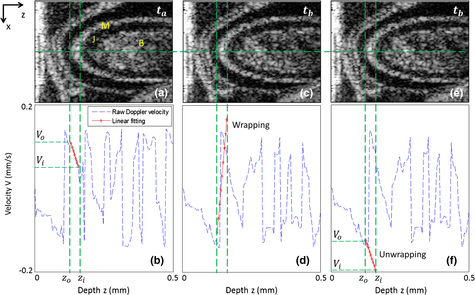

Fig. 5

Evaluation of both radial SR of myocardial wall and Doppler velocity of blood flow over cardiac cycles by the use of only one M-B scan afforded by the ultrafast imaging system used in this study: (a) M-mode structural image superimposed with radial SR of the myocardial wall and Doppler velocity of blood flow; (b) Doppler velocity along the dashed yellow line in Fig. 2(c); (c) Radial SR. The dashed vertical line indicates the three phases of the OFT activities, i.e., 1) the opening of outflow cushions (from $t_0$ to $t_1$); 2) the start of atrioventricular (AV) ejection or closure of the AV cushions (from $t_1$ to $t_2$); and 3) the closure of outflow cushions (from $t_2$ to $t_3$). TC: thickening of myocardial wall; TN: thinning of myocardial wall; F: forward flow; B: backward flow. The vertical bar in (a) represents 200 μm and the horizontal bar indicates 0.2 s.

The blood flow velocity, $V_B$, was measured by the use of phase-resolved DOCT,^12,44 which uses the phase shift $\mathrm{\Delta }\varnothing$ between adjacent A-scans within B-scans to evaluate the flow velocity,

Eq. (5)

$$V_B(t)=\frac{\mathrm{\Delta }\varnothing (t){\lambda }_0}{4\pi n\tau }\times \frac{1}{\cos ({\alpha }_B)},$$

where $\tau$ is the time interval between adjacent A-scans, which is $\sim 5\mathrm{\mu s}$ in our study for an imaging speed of 184 kHz. Refer to Fig. 3(b), ${\alpha }_B$ is the Doppler angle when evaluating the flow velocity using OCT. Note that the phase information is used for the evaluation of either blood flow velocity or the tissue velocity, however, the phase angle is $2\pi$ modulo. Thus, considering that the refractive indices of the wall and the blood as 1.38, the maximum velocity without ambiguity that the proposed method can provide is $\sim 43.95\mathrm{mm}/\mathrm{s}$ for blood flow and $\sim 0.133\mathrm{mm}/\mathrm{s}$ for myocardial wall motion in both positive and negative directions.

Due to the fact that the motion direction is difficult to be assessed precisely in the fast beating heart, the Doppler angle correction was initially neglected in this study, i.e. assuming that ${\alpha }_M\approx 0$ and ${\alpha }_B\approx 0$. During experiments, attention was paid to ensure that the scanning plane, i.e. B-frame was approximately close to $90°$ (but $<90°$) to the longitudinal direction of the OFT, which can be judged by checking whether the OFT cross section is round when it is most expanded.

In the results present below, the negative sign indicates a thinning of the myocardial wall for SR or a backward blood stream for flow velocity, and the positive sign implies a thickening of the myocardial wall for SR or a forward blood stream for flow velocity. Here the term “backward” means blood is mainly moving toward the probing light or inward the ventricle from the OFT, while the term “forward” means blood is mainly moving away from the probing light or outward the ventricle to the OFT.

To facilitate the study, a software program was developed to automatically segment the myocardial wall from the M-mode structural image by the use of a deformable model based algorithm.⁴⁵ Briefly, the user manually traces the mid-line of the myocardial wall in the M-mode structural image. Then a 2-D deformable rectangular model (or double-line model) is used to find the boundaries of the myocardial wall by adjusting the distance between lines in the deformable model, using an M-estimator.⁴⁵ This procedure automatically adjusts the midline and extracts the outer and the inner boundaries of the myocardial wall. Interested readers should refer to Ref. 45 for details. The thickness of the myocardial wall is the distance between the two boundaries.

3.

Results and Discussion

Due to its high spatial resolution, OCT imaging is capable of resolving main microstructural elements within the OFT (see Fig. 2), including the blood (B) in the lumen, the myocardium (M), and the cardiac jelly (CJ) that forms endocardial cushions in the heart OFT. The endocardial cushions are protrusions of the heart walls toward the lumen (more specifically extra-cellular matrices) and limit backflow in the OFT when the myocardium contracts by closing the lumen area. Ultimately endocardial cushions will contribute to the formation of the intraventricular septum and will develop into semilunar valves.

The radial deformation (thickening and thinning) of the myocardial wall is visible in the M-mode structural image [Fig. 2(c)] along the time-dependent central A-line. The M-mode structural image was extracted from the time-lapse B-scan images at the dashed vertical line shown in Fig. 2(a) (an OFT longitudinal section) or Fig. 2(b) (an OFT cross-section). From the M-mode structural image the myocardial wall was automatically identified using our segmentation algorithm [refer to solid curves in Fig. 2(c)], from which the boundary positions of the myocardial wall were extracted [Fig. 2(d)]. Accordingly, the thickness variation of the myocardial wall was obtained [Fig. 2(e)], with an accuracy that is determined both by the axial resolution of the OCT system used ($\sim 8.7\mathrm{\mu m}$), the contrast in the image, and the accuracy of the segmentation algorithm. For this case, the thickness of the myocardial wall was $\sim 25\mathrm{\mu m}$ when the OFT was most expanded, and $\sim 53\mathrm{\mu m}$ when OFT was most contracted. Because the M-mode image consisted of 1000 repeated B-scans captured at the speed of 560 fps, it can be seen from the results that the heart rate in this study was $\sim 1.73\text{beats per second}$ (cardiac period $\sim 0.58\mathrm{s}$).

From these evaluations, the approximate SR of the myocardial wall during one cardiac cycle was approximated to $\pm 1.82{\mathrm{s}}^{-1}$. Note that the approximate SR can be evaluated by $\frac{\text{thickness change}}{\text{orginal thickness}\times \text{half cardiac period}}$. The heart rate of 1.73 is a little lower than that in normal case that should be $\sim 2.2$ to $2.4\text{beats per second}$. This was most likely due to the fact that imaging was performed under room temperature. In our future studies, precautions will be taken to precisely control the experimental temperature so that the dynamic interaction between the cardiac wall and the flowing blood can be systematically studied under physiological environment.

Figure 4 shows the representative tissue-Doppler velocity profiles evaluated at the central A-line position (the dashed horizontal lines in the structural images) by using Eq. (4) at two time instants. Because the phase-shift between adjacent B-scans was used, the maximal tissue velocity that the approach can provide without ambiguity was $\pm 0.133\mathrm{mm}/\mathrm{s}$ with $T=1.78\mathrm{ms}$ (if the refractive index of the tissue is taken as 1.38). This velocity limit makes the evaluated velocity profile look quite noisy throughout the depth profile. However, the velocity of the cardiac wall is generally slow, and its corresponding tissue phase is stable. To facilitate the evaluation of the SR of the cardiac wall, the structural wall boundary (e.g., Fig. 4) was used to locate the cardiac wall within Doppler velocity profile. This is shown as a paired image of Fig. 4(a) and 4(b), where the velocity signal from the cardiac wall is marked as red. As shown, the depth-dependent velocity within the myocardial wall is generally linear, which is in good agreement with the assumption of the linear distribution of the wall velocity.³⁴ Due to the limitation of maximal velocity ($0.133\mathrm{mm}/\mathrm{s}$), any velocity faster than this value would cause phase wrapping when evaluating the phases from the complex OCT signals because of $2\pi$ phase modulo. This is the case for Fig. 4(c) and 4(d), where the wall motion exceeded $0.133\mathrm{mm}/\mathrm{s}$. To recover the true tissue velocity, a phase unwrapping algorithm was applied to automatically correct the phase wrapping [Fig. 4(f)].⁴⁶ This way doubles the measurable wall motion speed to $0.266\mathrm{mm}/\mathrm{s}$, which is sufficient for almost all of our cases. After correction of all tissue velocity values, the radial SR of the myocardial wall, i.e. the slope of the velocity versus depth, is readily obtainable through the linear fitting to the velocity profile bounded by the wall boundaries defined by the OCT microstructural images.

After the segmentation of cardiac wall boundaries and proper treatment of phase wrapping (if any) to arrive at the correct velocity profile corresponding to the wall motion, the time-dependent radial SR and blood flow velocity can be evaluated. Figure 5 reports such results evaluated along the dashed line shown in Fig. 2(c) over approximately three cardiac cycles, overlaid on top of the corresponding M-mode structural image for easy comparison.

It is observed that, there existed three peaks within each cardiac cycle for the Doppler velocity profile of blood flow. These peaks include a backward flow peak $P_1$ and two forward flow peaks $P_2$ and $P_2$ as marked in Fig. 5(b). These observations are consistent with those reported in prior studies^47–49 where however the Doppler ultrasound was used to characterize the blood flow within the developing embryonic heart. According to the studies in Refs. 47 to 49, the first peak, corresponding to the backward flow $P_1$, was due to the opening of the outflow cushions which gives rise to sucking of blood towards the ventricle; the second peak, corresponding to the forward flow $P_2$, was due to the closure of the atrioventricular (AV) cushions and blood ejection from the ventricle; and the third peak, the forward flow peak $P_3$, was induced by contractile motion of the OFT walls.

Therefore from the observations in the current results compared with those reported in prior studies,^47–49 the periodically dynamic interactions between the myocardial wall and the flowing blood can be approximately divided into three phases, i.e., phase I indicates the opening of the OFT lumen (from $t_0$ to $t_1$); phase II represents the beginning of ventricular ejection (from $t_1$ to $t_2$); and phase III corresponds to the closing of the lumen (from $t_2$ to $t_3$). More specifically, the three phases can be explained as below:

It is noted in Fig. 5(c) that, during a cardiac cycle, the instant SR varied from $-2.2$ to $2.4{\mathrm{s}}^{-1}$. This range is generally in good agreement with that evaluated from the OCT structural imaging (see Fig. 2), which was estimated within a range of $\pm 1.82{\mathrm{s}}^{-1}$. The underestimation of the latter method is likely due to that the accuracy in the estimation of wall thickness because it is limited by the axial resolution of the imaging system, which is $\sim 8.7\mathrm{\mu m}$ in tissue. This demonstrates the proposed method may offer potential advantage over the conventional OCT approach in assessing the dynamic wall motion.

It is also noted in Fig. 5(c) that there appeared some large fluctuations in the time-dependent SR curve during phase II when OFT was most expanded. This fluctuation was most likely attributed to the reasons that: 1) When OFT was most expanded, the wall thickness was thin ($\sim 4\text{pixels}$). Thus the accuracy of the myocardial wall segmentation becomes important when the linear fitting was applied to extract the radial SR from a limited number of available points. In this case, higher pixel resolution would be required to increase the accuracy.³⁴ 2) As shown in Fig. 5(b), during this phase, the rapid AV ejection would introduce a large bulk motion of OFT. Because of the relatively long time interval between the adjacent B-scans, such bulk motion reduced the spatial correlation between the adjacent B-scans that were used for the phase shift evaluation, resulting in measurement errors.

In order to evaluate the influence of the Doppler angles on the radial SR of the myocardial wall and the velocity of the flowing blood, the MB-mode OFT longitudinal sections were averaged over $\sim 3$ cardiac cycles. The result is shown in Fig. 6, where it can be seen that the Doppler angle due to the radial deformation of the myocardial wall ${\alpha }_M$ is generally less than 10°. Thus the influence of the Doppler angle on the radial SR can be neglected. However, the Doppler angle ${\alpha }_B$ due to the blood flow within the lumen is between 70 and 80°. With such a Doppler angle, the magnitude of the velocity of the flowing blood as measured by the OCT should be corrected by multiplying a factor of 2.9 to 5.8. Please note that such Doppler angle correction for the flow velocity does not affect the velocity waveform as shown in Fig. 5. Therefore, the results and discussions presented above are still valid. In future, efforts will be paid to correct the Doppler angle effect on these measurements; for example, using sophisticated 4-D tracking algorithms,⁴ so that accurate characterization of the dynamic interactions between the myocardial wall and the flowing blood can be performed.

Fig. 6

Averaged OFT longitudinal sections for Doppler angle correction vertical scale bar = 200 μm.

4.

Conclusion

We have demonstrated that the dual-camera SDOCT system with $\sim 184\text{-}\mathrm{kHz}$ scanning rate provides enough flexibility to quantify the fast blood flow and the slow myocardial wall deformation of embryonic chick heart within one MB scan. The ability of simultaneous evaluation of these two important parameters in a developing heart offers an attractive means for characterizing the dynamic interactions between the myocardial wall and the flowing blood.