Comparative study of differential matrix and extended polar decomposition formalisms for polarimetric characterization of complex tissue-like turbid media

Satish Kumar; Harsh Purwar; Razvigor Ossikovski; I. Alex Vitkin; Nirmalya Ghosh

doi:10.1117/1.JBO.17.10.105006

12 October 2012 Comparative study of differential matrix and extended polar decomposition formalisms for polarimetric characterization of complex tissue-like turbid media

Satish Kumar, Harsh Purwar, Razvigor Ossikovski, I. Alex Vitkin, Nirmalya Ghosh

Author Affiliations +

Journal of Biomedical Optics, Vol. 17, Issue 10, 105006 (October 2012). https://doi.org/10.1117/1.JBO.17.10.105006

Abstract

Development of methodologies for quantification/unique interpretation of the intrinsic polarimetry characteristics of biological tissues are important for various applications involving tissue characterization/diagnosis. A detailed comparative evaluation of the polar decomposition and the differential matrix decomposition of Mueller matrices for extraction/quantification of the intrinsic polarimetry characteristics (with special emphasis on linear retardance δ , optical rotation Ψ and depolarization Δ parameters was performed, because these are the most prominent tissue polarimetry effects) from complex tissue-like turbid media exhibiting simultaneous scattering and polarization effects. The results suggest that for media exhibiting simultaneous linear retardance and optical rotation polarization events, the use of retarder polar decomposition with its associated analysis which assumes sequential occurrence of these effects, results in systematic underestimation of δ and overestimation of Ψ parameters. Analytical relationships between the polarization parameters (δ , Ψ ) extracted from both the retarder polar decomposition and the differential matrix decomposition for either simultaneous or sequential occurrence of the linear retardance and optical rotation effects were derived. The self-consistency of both decompositions is validated on experimental Mueller matrices recorded from tissue-simulating phantoms (whose polarization properties are controlled, known a-priori, and exhibited simultaneously) of increasing biological complexity. Additional theoretical validation tests were performed on Monte Carlo-generated Mueller matrices from analogous turbid media exhibiting simultaneous depolarization (Δ ), linear retardance (δ ) and optical rotation (Ψ ) effects.

1. Introduction

Mueller matrix polarimetry has received considerable recent attention for the characterization of a wide range of optical media for numerous practical applications in various branches of science and technology.¹^–³ The Mueller matrix (a $4 \times 4$ matrix) represents the transfer function of an optical system in its interactions with polarized light and contains complete information about the medium polarization properties.¹^–³ Mueller matrix polarimetry thus offers the possibility of quantifying the polarimetry characteristics (which contain wealth of morphological, structural and functional information) of the sample. However, complexities arise when more than one polarization effects occur within the sample (the three basic medium polarization properties being diattenuation, retardance and depolarization²) as these contribute in a complex interrelated way to the Mueller matrix elements, masking potentially interesting polarization metrics and hindering their unique interpretation.⁴ Quantitative polarimetry is further compromised due to the presence of strong multiple scattering effects in optically thick (turbid) media such as biological tissues.⁴^,⁵ Multiple scattering within a tissue not only causes extensive depolarization, but also alters the polarization state of the residual polarization-preserving signal in a complex fashion.⁴^,⁶ Each of the intrinsic polarization properties, if separately extracted from the ‘lumped’ system Mueller matrix, can potentially serve as a useful biological metric. For example, the anisotropic organized nature of many tissues stemming from their fibrous structure leads to linear retardance (or linear birefringence) effect. Changes in this anisotropy resulting from disease progression or treatment response alter the linear retardance properties, making this a potentially sensitive probe of tissue status.⁷^,⁸ Similarly, measurement and quantification of circular retardance (or optical rotation) may offer an attractive approach for noninvasive monitoring of tissue glucose levels.⁹

Various kinds of Mueller matrix decompositions have therefore been proposed in the recent past for inverse polarimetry analysis.¹⁰^–¹³ Among these, the product decomposition proposed by Lu and Chipman has been the most widely explored method.¹⁰ This method consists of decomposing a given Mueller matrix into sequential product of the three ‘basis’ matrices describing the three basic medium polarization properties, depolarization, retardance (linear and circular) and diattenuation (linear and circular). Since the product decompositions¹⁰^–¹³ model the resultant polarization processes as a preferred sequential product of the ‘basis’ matrices describing the constituent polarization effects, they are potentially ambiguous with respect to the order of the basis matrices, due to the noncommuting nature of matrix multiplication. Moreover, in complex systems like tissues, no unique order (or sequence) can be assigned to the polarimetry effects; rather, these are exhibited simultaneously. The decomposition-derived polarization parameters are thus expected to be influenced by the choice of the ordering of the basis matrices. Although our recent studies have shown that under certain conditions, the ambiguity in the decomposition-derived polarization parameters can be minimal,¹⁴ a more generally applicable inverse analysis model is certainly required for polarized light assessment of media exhibiting simultaneous polarization effects (such as tissues). In order to address this issue, a more general kind of decomposition based on differential matrix formalism of the Mueller calculus, has recently been developed.¹⁵^,¹⁶ This formalism, historically stemming from Jones $N$ -matrix formalism,¹⁷ was originally proposed by R. M. A Azzam for nondepolarizing optical media;¹⁸ it has been extended and generalized to incorporate depolarization effects.¹⁵ Within the differential matrix formalism, all elementary polarization and depolarization properties of the medium are contained in a single differential matrix representing them simultaneously. Thus, this approach is expected to be more suitable for Mueller matrix polarimetry analysis of tissues, exhibiting simultaneous polarization effects. Implementation of these approaches for polarized light assessment of complex systems like tissues would, however, require comprehensive validation. Specifically, it is necessary to perform a comparative evaluation of the polarization parameters derived via the differential matrix decomposition and the product decompositions (specifically, the widely used Lu-Chipman polar decomposition), and to establish a link between them. We have therefore investigated this issue by performing a detailed comparative evaluation of the polar decomposition and the differential matrix decomposition of Mueller matrices from complex tissue-like turbid media exhibiting simultaneous scattering and polarization effects. We have paid particular attention on linear retardance ( $δ$ ), optical rotation ( $Ψ$ ) and depolarization ( $Δ$ ) parameters, because these are the most prominent tissue polarimetry effects, which also hold promise as useful biological metrics for applications involving tissue characterization/diagnosis.⁴

In particular, we have studied the effect of simultaneous or sequential exhibition of linear retardance and optical rotation polarization events on the derived values for the $δ$ and $Ψ$ parameters using either the retarder polar decomposition (which assumes preferred sequential occurrence of these effects) or the differential matrix decomposition. In order to establish self-consistency, we have also derived analytical relationships between the polarization parameters ( $δ$ , $Ψ$ ) extracted from both the retarder polar decomposition and the differential matrix decomposition for either simultaneous or sequential occurrence of the linear retardance and optical rotation effects. The self-consistency of both decompositions is validated on experimental Mueller matrices recorded from tissue-simulating phantoms (whose polarization properties are controlled, known a-priori, and exhibited simultaneously) of increasing biological complexity. Additional theoretical validation tests were performed on Monte Carlo (MC)-generated Mueller matrices from analogous turbid media exhibiting simultaneous depolarization ( $Δ$ ), linear retardance ( $δ$ ) and optical rotation ( $Ψ$ ) effects. Finally, after successful evaluation, the potential advantages of the differential matrix decomposition over the previously used polar decomposition was explored for monitoring of myocardial tissue regeneration following stem cell therapy (through quantification of linear retardance obtained from the measured Mueller matrices). The results of these investigations are reported here.

The paper is organized as follows. In Sec. 2, we briefly summarize the mathematical methodology for polar decomposition and differential matrix decomposition of Mueller matrix for extraction of the constituent polarimetry characteristics. The derived conversion relations for the polarization parameters extracted from the two different decomposition formalisms are presented in this section. The analytical extension for ‘self-consistent’ extraction of linear retardance $δ$ and optical rotation $Ψ$ from both the decomposition formalisms for either simultaneous or sequential occurrence of the polarization events is also presented in this section. Section 3 briefly describes our experimental turbid polarimetry systems, optical phantoms and forward polarization sensitive Monte Carlo (MC) simulation model. The results of the comparative evaluation of polar decomposition and differential matrix decomposition and validation of the self-consistency of our extended formalisms on experimental Mueller matrices from phantoms and MC-generated Mueller matrices are presented in Sec. 4. Selected experimental results on the use of differential matrix decomposition from myocardial tissue samples are then presented, interpreted and discussed. The paper concludes with a discussion on the potential advantages of the differential matrix decomposition in quantitative polarimetric tissue characterization/diagnosis.

2. Theory

2.1.

Polar Decomposition of Mueller Matrix

Polar decomposition method consists of decomposing a given Mueller matrix $M$ into the sequential product of three ‘basis’ matrices,

Eq. (1)

M \Leftarrow M_{Δ} . M_{R} . M_{D},

with

\Leftarrow

symbol used to signify the decomposition process. Here, the matrix

M_{Δ}

describes the depolarizing effects of the medium,

M_{R}

accounts for the effects of linear and circular retardance (or optical rotation), and

M_{D}

includes the effects of linear and circular diattenuation. This product decomposition with multiplication order of Eq. (1) was proposed by Lu and Chipman and is accordingly known as Lu-Chipman decomposition.¹⁰ Once calculated, these constituent basis matrices are further analyzed to derive individual polarization medium properties. Specifically, diattenuation (

D

), depolarization coefficient (

Δ

), linear retardance (

δ

), and circular retardance/optical rotation (

Ψ

) (

circular retardance = 2 \times optical rotation

), can be determined from the decomposed basis matrices as shown below.

The magnitude of diattenuation ( $D$ ) can be determined from the diattenuation matrix $M_{D}$ as¹⁰

Eq. (2)

D = \frac{1}{M_{D} (1, 1)} \sqrt{M_{D} {(1, 2)}^{2} + M_{D} {(1, 3)}^{2} + M_{D} {(1, 4)}^{2}} .

Net depolarization coefficient

Δ

is quantified through the depolarization matrix

M_{Δ}

as¹⁰

Eq. (3)

Δ = 1 - \frac{| tr (M_{Δ}) - 1 |}{3}, 0 \leq Δ \leq 1.

Assuming sequential effects of linear retardance and optical rotation the retarder matrix $M_{R}$ can be further decomposed into what can be termed “retarder polar decomposition,”

Eq. (4)

M_{R} \Leftarrow M_{L} \cdot M_{C} = M_{C} \cdot M_{L},

where

M_{C}

and

M_{L}

(

M_{L}

) are another two retarder matrices exhibiting only circular (i.e., optical rotation) and linear retardance, respectively.⁶^,¹⁹ By inserting the standard Mueller matrix forms for linear and circular retarders²^,¹⁹ into [Eq. (4)], the magnitudes of linear retardance

δ

and optical rotation

Ψ

can be calculated directly from the elements of the retarder matrix

M_{R}

as ⁶^,¹⁹

Eq. (5)

δ = \cos^{- 1} {\sqrt{[M_{R} (2, 2) + M_{R} {(3, 3)]}^{2} + {[M_{R} (3, 2) - M_{R} (2, 3)]}^{2}} - 1}

Eq. (6)

Ψ = \tan^{- 1} [\frac{M_{R} (3, 2) - M_{R} (2, 3)}{M_{R} (2, 2) + M_{R} (3, 3)}] .

Note that the magnitudes $δ$ and $Ψ$ of linear retardance and optical rotation do not depend on their order of appearance in the sequence although the matrix product is generally noncommutative. The total retardance $R$ (a parameter that represents the combined effect of linear and circular retardance) can also be determined from $M_{R}$ ¹⁰^,¹⁹

Eq. (7)

R = \cos^{- 1} {\frac{Tr (M_{R})}{2} - 1} .

An algorithm for decomposing Mueller matrices with multiplication order of the basis matrices reverse to that of Eq. (1) has also been developed (reverse decomposition¹¹), and it has been shown that all other possible decompositions (a total number of six depending upon the order of multiplication) can be obtained from these two decompositions by using similarity transformations.¹¹ Note, although, that the processes for decomposition using the order of Eq. (1) or its reverse order are qualitatively similar; there do exist subtle differences in the construction of the basis matrices and the derived polarization parameters.¹¹ Never-the-less all families of product decompositions model the polarized light–matter interaction as a sequential product (of unique order or sequence) of the basis matrices describing the constituent polarization effects, and are thus potentially ambiguous with respect to the multiplication order of these matrices.

2.2.

Differential Matrix Decomposition

Within the differential matrix formalism, the elementary properties of the medium are contained in the differential matrix $m$ which is related to the Mueller matrix $M$ and its spatial derivative along the propagation of light as

Eq. (8)

\frac{d M}{d Z} = m M .

The physical picture behind Eq. (8) assumes that the medium is laterally homogeneous (at least within the spot dimension of the probing light) and that the polarization and depolarization effects take place simultaneously.¹⁸ The general form of the differential matrix

m

for depolarizing anisotropic media in terms of basic properties of the medium is given by Ref. 15

Eq. (9)

m = (\begin{matrix} α & β & γ & \partial \\ β^{'} & α_{1} & μ & - ν \\ γ^{'} & - μ^{'} & α_{2} & η \\ \partial^{'} & ν^{'} & - η^{'} & α_{3} \end{matrix}) .

Here, $β$ and $γ$ is the linear dichroism along $x y$ (horizontal- vertical) and $\pm 45 °$ laboratory axes, respectively; $\partial$ is the circular dichroism; $η$ and $ν$ are linear birefringence along $x y$ and $\pm 45 °$ axes, respectively; $μ$ is the circular birefringence; $α$ and $α_{1}$ , $α_{2}$ , $α_{3}$ , respectively are the isotropic absorption and the anisotropic absorptions (or depolarizations) along $x y$ $\pm 45 °$ and circular axes, respectively. Note that in absence of depolarization, $α = α_{1} = α_{2} = α_{3} (= 0)$ . Moreover, in such case, $(β^{'}, γ^{'}, \partial^{'}, η^{'}, ν^{'}, μ^{'}) = (β, γ, \partial, η, ν, μ)$ . In the general case of a depolarizing medium, the six elementary polarization properties are in fact, the mean values of the corresponding pairs $(β, β^{'})$ , $(γ, γ^{'})$ , $(\partial, \partial^{'})$ , $(η, η^{'})$ , $(ν, v^{'})$ and $(μ, μ^{'})$ .¹⁵

If the medium properties (both polarizing and depolarizing) are uniformly distributed along the propagation direction $Z$ , i.e., the differential matrix $m$ is $Z$ -independent, Eq. (8) can be integrated to yield

Eq. (10)

L = \ln M = m l,

with

L

being the matrix logarithm of

M

and

l

being the optical pathlength, i.e., the equivalent length light would travel in the medium if optical properties and depolarization occurred truly simultaneously and were perfectly uniformly distributed longitudinally. If these conditions are met in practice, then

l

can be identified either with the sample thickness in case of forward scattering experiment or with the penetration depth in backscattering geometry. (It should be noted for completeness that Mueller matrix logarithm decomposition, Eq. (10), is formally equivalent²⁰ to the matrix roots decomposition that has been introduced by Chipman,²¹ thus initiating the differential (simultaneously occurring properties) decomposition approach, in contrast to the product, (sequentially occurring properties) one.

The elementary properties of the medium can be determined by constructing the Lorentz antisymmetric, $L_{m}$ , and symmetric, $L_{u}$ , components of $L (L = L_{m} + L_{u})$ as follows¹⁵

Eq. (11)

L_{m} = \frac{1}{2} (L - G L^{T} G) and L_{u} = \frac{1}{2} (L + G L^{T} G),

where

G = diag

(1,

- 1

,

- 1

,

- 1

) is the Minkowski metric tensor.

For a depolarizing medium, the off-diagonal elements of $L_{m}$ represent the mean values of the six elementary properties [as per Eq. (9)] accumulated over pathlength $l$ , while the off-diagonal elements of $L_{u}$ express their respective uncertainties. Further, the main diagonal elements of the matrix $L_{u}$ ( $α_{1}$ , $α_{2}$ and $α_{3}$ ) represent the depolarization coefficients (after the subtraction of the isotropic absorption $α$ from the diagonal) along the $x y$ , $\pm 45 °$ and circular axes.¹⁵ The accumulated polarization parameters (intrinsic properties scaled by pathlength $l$ ) can be determined from the elements of the $L_{m}$ and $L_{u}$ matrices as

Eq. (12)

Net dichroism d = \sqrt{{[L_{m} (1, 2)]}^{2} + {[L_{m} (1, 3)]}^{2} + {[L_{m} (1, 4)]}^{2}}

Eq. (13)

Net depolarization Δ_{m} = \frac{1}{3} | α 1 + α 2 + α 3 |

Eq. (14)

Linear retardance δ^{\log - M} = \sqrt{{[L_{m} (2, 4)]}^{2} + {[L_{m} (3, 4)]}^{2}}

Eq. (15)

Optical rotation Ψ^{\log - M} = \frac{1}{2} L_{m} (2, 3)

The angle of orientation of the axis of linear retardance is

Eq. (16)

θ^{\log - M} = \frac{1}{2} \tan^{- 1} \frac{{L_{m} (2, 4)}}{{L_{m} (3, 4)}} .

In this convention, the total retardance can be determined as

Eq. (17)

R^{\log - M} = \sqrt{{(δ^{\log - M})}^{2} + {4 (Ψ^{\log - M})}^{2}} .

Note that the uncertainties (standard deviations) of the parameters, diattenuation, linear retardance and optical rotation (and total retardance) can also be derived employing the same set of Eqs. (12, 14, 15, and 17) on the off-diagonal elements of the matrix

L_{u}

. As we shall see later, the derived standard deviations of these parameters contain additional useful information on the randomness (random organization of diattenuation and retardance) of the medium.

2.3.

Conversion Relations for the Polarization Parameters

An important issue while relating the medium polarimetry characteristics defined in the polar decomposition formalism [Eqs. (2)–(7)] and those in the differential matrix formalism (the accumulated polarization parameters defined in Eqs. (12)–(17), is the conversion from one set of parameters to the other. Note that the Mueller matrix corresponding to each accumulated polarization parameter (elements of the differential matrix $m$ scaled by pathlength $l$ ) can be obtained from the solution of Eq. (8) and the eigenvalues of $m$ .¹⁸^,²² From these derived Mueller matrices (for each of the polarization effects) and the corresponding known forms of Mueller matrices in the polar decomposition formalism,²^,⁴ one can derive the following relations.

Eq. (18)

D^{\log - M} = \tanh (d) = \tanh {\sqrt{{[L_{m} (1, 2)]}^{2} + {[L_{m} (1, 3)]}^{2} + {[L_{m} (1, 4)]}^{2}}} \leftrightarrow D^{polar},

Eq. (19)

Δ^{\log - M} = 1 - \frac{1}{3} (e^{- α_{1}} + e^{- α_{2}} + e^{- α_{3}}) \leftrightarrow Δ^{polar},

where the double arrow (“

\leftrightarrow

”) stands for “numerically comparable to.” Note that the above two conversion relations between the differential matrix formalism and the polar decomposition formalism represent diattenuation

D

and depolarization

Δ

within the same limiting values (magnitude between 0 and 1). More precisely, Eq. (18) transforms dichroism into diattenuation while Eq. (19) converts the three logarithmic depolarization coefficients into a single “conventional” net depolarization. However, no such conversion is required for retardance (either linear or circular).

2.4.

Analytical Extension for “Self-Consistent” Extraction of Linear Retardance $δ$ and Optical Rotation $Ψ$

Having discussed the normalization criteria for diattenuation and depolarization effects, we now turn our attention to the important issue of self-consistent determination of linear retardance $δ$ and optical rotation $Ψ$ using differential matrix decomposition and the retarder polar decomposition [(Eq. 4)], for either simultaneous or sequential effects. The form of a Mueller matrix exhibiting simultaneous linear retardance and circular retardance can be derived, from the differential matrix ( $L_{R}$ ) representing a retardance effect alone, as $M_{R} = \exp (L_{R})$ yielding¹⁸^,²²

Eq. (20)

M_{R} = (\begin{matrix} 1 & 0 & 0 & 0 \\ 0 & \cos R + η^{2} ρ & - η ν ρ + μ σ & - η μ ρ - ν σ \\ 0 & - η ν ρ - μ σ & \cos R + ν^{2} ρ & ν μ ρ - η σ \\ 0 & - η μ ρ + ν σ & ν μ ρ + η σ & \cos R + μ^{2} ρ \end{matrix}),

where

R

is the total retardance (

R = \sqrt{η^{2} + ν^{2} + μ^{2}}

);

ρ

and

σ

are defined as

ρ = (1 - \cos R) / R^{2}

and

σ = \sin R / R

and the differential matrix

L_{R}

representing retardance effect alone, is¹⁸

Eq. (21)

L_{R} = (\begin{matrix} 0 & 0 & 0 & 0 \\ 0 & 0 & μ & - ν \\ 0 & - μ & 0 & η \\ 0 & ν & - η & 0 \end{matrix}) .

Once again, the values of the polarization parameters entering the various elements of

L_{R}

(and thus, those of

M_{R}

also) are accumulated values over the pathlength

l

. It is obvious that determination of linear retardance (

δ

) and optical rotation (

Ψ

) employing Eqs. (5) and (6)—in the retarder polar decomposition formalism [Eq. (4)]–from the elements of the Mueller matrix of Eq. (20), would lead to erroneous estimation of these parameters since the Mueller matrix derived using sequential multiplication of Mueller matrices for pure linear retarder and optical rotation is generally not the same as that of Eq. (20) representing simultaneous occurrence of these effects.²^,¹⁸ However, as is obvious from Eqs. (7), (17), and (20), the value of total retardance (

R

) would remain the same. This discrepancy in determination of

δ

and

Ψ

parameters can be rectified, if these are directly estimated from the elements of the retardance vector introduced below.

The elements of the retardance vector $\vec{R} = R {(r_{1}, r_{2}, r_{3})}^{T}$ can be derived from the $3 \times 3$ submatrix $m_{R}$ of the $4 \times 4$ retardance matrix $M_{R}$ obtained via the polar decomposition (first column) as¹⁰

Eq. (22)

r_{i} = \frac{1}{2 \sin R} \sum_{}^{} ε_{i j k} {(m_{R})}_{j k},

where

ε_{i j k}

is the Levi—Civita permutation symbol and

M R = (\binom{1}{\vec{0}} \binom{\vec{0}}{m_{R}})

.

Using Eqs (20) and (22), the elements of the retardance vector can be determined as

Eq. (23)

\vec{R} = R {(r_{1}, r_{2}, r_{3})}^{T} = {(η, ν, μ)}^{T} .

This shows the equivalence between the two approaches when the retardance effects (linear retardance and optical rotation) occur simultaneously. The values for net linear retardance $δ$ and optical rotation $Ψ$ can thus be determined with the help of Eqs. (14) and (15) as

Eq. (24)

δ (simult aneous) = R \sqrt[]{r_{1}^{2} + r_{2}^{2}},

Eq. (25)

Ψ (simult aneous) = \frac{R r_{3}}{2},

rather than from Eqs. (5) and (6) based on the retarder polar decomposition.

The validity of the determination of $δ$ and $Ψ$ parameters using Eqs. (24) and (25) in combination with polar decomposition has been tested on experimental Mueller matrices from optical phantoms exhibiting simultaneous linear retardance, optical rotation and depolarization effects and on analogous MC-generated Mueller matrices. These results are presented subsequently.

Conversely, when the medium exhibits sequential linear and circular retardance effects the use of differential matrix formalism—Eqs. (14) and (15)–would yield erroneous estimation of $δ$ and $Ψ$ parameters for the same reason described above. In fact, the differential matrix formalism can also be ‘corrected’ to yield the ‘true’ values for $δ$ and $Ψ$ , even for sequential occurrence of these effects. Here, the correction process is based on determination of these parameters from the eigenvalues and the eigenvectors of the differential matrix for the retardance alone, $L_{R}$ . [ $L_{R}$ is derived from the Lorentz antisymmetric component $L_{m}$ of the matrix logarithm $L$ of the experimental Mueller matrix; see Eqs. (10) and (11)] The eigenvalues of the matrix $L_{R}$ are (0, 0, $i R$ , $- i R$ ), whereas one of the eigenvectors corresponding to the doubly degenerate zero eigenvalue turns out to be the vector ${(1, r_{1}, r_{2}, r_{3})}^{T}$ i.e., its last three components are proportional to the retardance vector $\vec{R}$ . Using the known forms of linear retarder and optical rotation matrices²^,⁴ and assuming sequential effects (of either order), the analytical formulations of the components of $\vec{R}$ can be derived. Following a series of algebraic manipulations, sequentially occurring linear retardance $δ$ and optical rotation $Ψ$ can be related to the components of the retardance vector (i.e., to the eigenvector of $L_{R}$ ) as

Eq. (26)

δ (sequen tial) = 2 \sin^{- 1} \sqrt{(r_{1}^{2} + r_{2}^{2}) \frac{1 \pm \sqrt{1 - \sin^{2} R}}{2}}

Eq. (27)

Ψ (sequen tial) = \frac{1}{2} \sin^{- 1} \frac{2 r_{3} \sin R}{1 + \cos δ},

where the value for total retardance

R

can be directly determined from the two nonzero eigenvalues of

L_{R}

. The positive and negative signs in Eq. (26) are for

R < π / 2

and for

R > π / 2

, respectively.

The analytical relationships provided above allows one to self consistently extract the values of linear retardance $δ$ and optical rotation $Ψ$ from both decomposition formalisms for either simultaneous or sequential occurrence of these polarization events. While we have focused our attention on the validation of the two formalisms for media exhibiting simultaneous polarization effects (because this is the situation typically encountered in tissues⁴), the validity of the determination of $δ$ and $Ψ$ parameters using Eqs. (26) and (27) with differential matrix decomposition for the sequential occurrence of linear and circular retardance effects, is also warranted. It is also worth mentioning here that, in the differential matrix formalism, the total retardance (or birefringence) is represented in a basis using two linear ( $x y$ , horizontal–vertical, birefringence and $\pm 45 \deg$ birefringence) and one circular axis¹⁸^,²² whereas, in the polar decomposition formalism, retardance is generally represented by linear retardance $δ$ , its orientation angle $θ$ and circular retardance ( $2 Ψ$ ).¹⁰ By establishing a link between these two formalisms, the parameters of the differential matrix formalism are thus transformed to the latter representation basis, as is apparent from Eqs. (12)–(17).

3. Experimental Methods

3.1.

Experimental Polarimetry Systems

The experimental Mueller matrix polarimetry system employed in our study consists of both point measurement and imaging systems. The point polarimetry system employs polarization modulation with synchronous detection and thus provides a high signal-to-noise ratio (SNR) polarimetric signal. The imaging system employs $d c$ measurements involving sequential measurements with different combinations of source polarizers and detection analyzers, albeit with lower SNR than the synchronous $a c$ detection schemes. The imaging system, although suffering from a lower SNR, allows for spatial mapping of the polarization parameters of a sample.

The details of our point measurement polarimetry system have been reported previously.¹⁹^,²³ Briefly, our turbid-polarimetry system employs polarization modulation using a photoelastic modulator (Hinds Instruments IS-90) and synchronous lock-in detection (Stanford Research Systems, SR830), allowing sensitive low-noise measurements of the Stokes vector of light interacting with a turbid sample in various geometries.⁴^,¹⁹^,²³ In our experimental embodiment, we employ polarization modulation on the sample-emerging light by placing the polarization modulator (along with a removable quarter-wave plate and a linear analyzer) between the sample and the detector.⁴^,¹⁹ By cycling the polarization of the incident beam (He-Ne laser, 15 mW, $λ = 632.8 nm$ ) using a linear polarizer and quarter wave-plate combination, and measuring the output Stokes vectors ( $I$ , $Q$ , $U$ , $V$ ), the Mueller matrix of the sample can be constructed.¹⁹ The input polarization was sequentially cycled between four states (linear polarization at 0, 45, and 90 deg, and right circular polarization) and the output Stokes vector for each respective input states were measured. The Mueller matrix was constructed from the measured set of Stokes vectors as¹⁹

Eq. (28)

M (i, j) = [\begin{matrix} \frac{1}{2} (I_{H} + I_{V}) & \frac{1}{2} (I_{H} - I_{V}) & I_{p} - M (1, 1) & I_{R} - M (1, 1) \\ \frac{1}{2} (Q_{H} + Q_{V}) & \frac{1}{2} (Q_{H} - Q_{V}) & Q_{p} - M (2, 1) & Q_{R} - M (2, 1) \\ \frac{1}{2} (U_{H} + U_{V}) & \frac{1}{2} (U_{H} - U_{V}) & U_{p} - M (3, 1) & U_{R} - M (3, 1) \\ \frac{1}{2} (V_{H} + V_{V}) & \frac{1}{2} (V_{H} - V_{V}) & V_{p} - M (4, 1) & V_{R} - M (4, 1) \end{matrix}] .

Here, the four input states are denoted with the subscripts $H$ (0 deg), $P$ (45 deg), $V$ (90 deg), and $R$ (right circular). The indices $i$ , $j = 1$ , 2, 3, 4 denote rows and columns, respectively.

In the imaging polarimetry system, light from a 635-nm diode laser (ThorLabs) was used as the excitation source. The polarization state of the incident light is controlled using a removable quarter-wave plate and a linear polarizer (forming a polarization state generator, PSG). As the beam exits the sample, a removable quarter-wave plate and linear analyzer (polarization state analyzer, PSA) select a single polarization state of the outgoing light, which is finally detected with a CCD camera (CoolSNAP K4, Photometrics, $2048 \times 2048 pixels$ , $7.4 \times 7.4 {μ m}^{2} pixel$ size). Four input states (horizontal 0 deg, vertical 90 deg, $+ 45$ , right-circularly polarized) and six output states (horizontal, vertical, $\pm 40$ deg, right- and left circularly polarized light) were recorded for a total of 24 combinations of measurements. The output Stokes parameters for each input state were measured from the detected intensities as²⁴

Eq. (29)

I = I_{0^{°}} + I_{90^{°}} Q = I_{0^{°}} - I_{90^{°}} U = I_{+ 45 °} - I_{- 45 °} V = I_{R} - I_{L},

where the subscripts indicate the output state being detected (as determined by the presence or absence of the quarter-wave plate, and the orientation of the analyzer). Finally, the 16 elements of the Mueller matrix were determined using Eq. (28) in a manner similar to that for the point measurement system.

Solid polyacrylamide phantoms were used as tissue simulating phantoms in our study. These solid optical phantoms were developed using polyacrylamide as a base medium, with sucrose-induced optical activity, polystyrene microspheres-induced scattering and mechanical stretching to cause linear birefringence.¹⁹ These phantom systems mimic the complexity of biological tissues, in that they exhibit simultaneous effects of linear birefringence, optical activity and depolarization due to multiple scattering. Transmission Mueller matrices from these phantoms were recorded using the point measurement polarimetry system.¹⁹^,²³ To investigate the utility of linear retardance measurements and quantification (using differential matrix decomposition) for monitoring regenerative treatments, samples from a rat model of myocardial infarction and regeneration were used.²³^,²⁴ All animal studies were carried out under institutional approval from the University Health Network, Toronto, Canada. Myocardial infarctions were induced in Lewis rats through coronary artery ligation. A group of animals was used as a control and mesenchymal stem cells were administered to a treatment groups by intra-myocardial injection into the site of infarction, two weeks post ligation. Both control and treatment groups were sacrificed four weeks post infarction (two weeks post stem-cell injections for the two treatment groups), at which time the hearts were removed, fixed in 10% formalin, and sectioned to one-mm-thick axial sections. Mueller matrix images were recorded in the transmission geometry, from these 1-mm-thick ex vivo tissue samples.²⁴

3.2.

Forward Polarization Sensitive Monte Carlo Simulation Model

We have used the polarization sensitive Monte Carlo (PSMC) model developed and validated previously by our group,²⁵ to generate Mueller matrices from the simulated turbid media exhibiting simultaneous linear birefringence, optical activity and depolarization effects (analogous to the optical phantoms). An important aspect of our PSMC model is that it has been extended²⁵ to simulate the simultaneous effects of linear birefringence and optical activity in the presence of multiple scattering, through the use of Jones’ $N$ -matrix formalism.¹⁷ This model thus mimics the experimental optical phantoms in that the polarization effects are exhibited in a simultaneous fashion over the path length of the simulated medium. The specifics of the model can be found in references.²⁵^,²⁶

Simulations were run for a set of input optical parameters of the scattering medium (scattering coefficient $μ_{s}$ , absorption coefficient $μ_{a}$ ) exhibiting simultaneous linear and circular birefringence effects. In the simulations, circular and linear birefringence was modeled through the optical activity $χ$ in degrees per centimeter, and through the anisotropy in refractive indices ( $Δ n$ ), respectively. Here, $Δ n (= n_{e} - n_{0})$ is the difference in refractive index along the extraordinary axis ( $n_{e}$ ) and the ordinary axis ( $n_{o}$ ). For simplicity, it was assumed that the direction of the extraordinary axis and the value for $Δ n$ is constant throughout the scattering medium. In each simulation, $n_{e}$ and $n_{o}$ were given as input parameters and a specific direction of the extraordinary axis was chosen. The Mueller matrices were generated for a slab of scattering medium having varying optical properties ( $μ_{s}$ , $Δ n$ and $χ$ ), for light exiting the medium through any user-selected direction.²⁶ The absorption was taken to be small ( $μ_{a} = 0.001 {cm}^{- 1}$ ) for all simulations. The photon collection geometry was chosen to have a detection area of $1 {mm}^{2}$ and an acceptance angle of 20 deg.

4. Results and Discussion

Figure 1 shows the results of the decomposition analysis on the $4 \times 4$ Mueller matrix experimentally recorded in the forward (transmission) detection geometry from a birefringent ( $extension = 4 mm$ for strain applied along the vertical direction), chiral (optical activity $χ = 1.96 \deg / cm$ , corresponding to 1 M concentration of sucrose), nonscattering phantom ( $μ_{s} = 0 {cm}^{- 1}$ ).¹⁹ The Mueller matrix logarithms $L_{m}$ and $L_{u}$ [derived via Eq. (10)] are shown and the estimated polarization parameters using both the differential matrix and polar decomposition approaches are also listed in the accompanying Table 1.

Fig. 1

Top: The experimentally recorded Mueller matrix (in the forward scattering geometry) and the corresponding $L_{m}$ and $L_{u}$ matrices for a birefringent ( $extension = 4 mm$ ), chiral ( $concentration of sucrose = 1 M$ , $χ = 1.96 \deg . {cm}^{- 1}$ ), nonscattering ( $μ_{s} = 0 {cm}^{- 1}$ ) p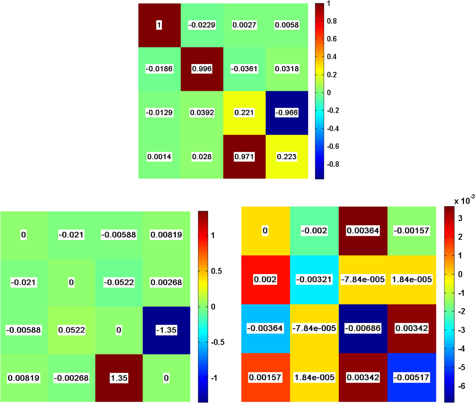hantom.

Table 1

The values for the polarization parameters extracted using Eqs. (14)–(19) (noted as Differential matrix, 2nd column). The values for the parameters extracted via retarder polar decomposition and its associated algebra [Eqs. (2)–(7)], which assumes sequential occurrence of linear retardance and optical rotation (retarder polar decomposition sequential, third column). The R, δ and Ψ-parameters extracted using Eqs. (23)–(25), for simultaneous δ and Ψ effects (retarder polar decomposition simultaneous [Eq. (4)]. The uncertainties of the parameters were calculated from the matrix lu. The uncertainty of the parameter Ψlog-M was very small (∼10−5) and hence not given.

Parameters	Differential matrix	Retarder polar decomposition (Sequential)	Retarder polar decomposition (Simultaneous)
$Δ$	0.005	0.005	0.005
$δ$ (radian)	$1.345 \pm 0.003$	1.345	1.345
$Ψ$ (radian)	0.026	0.031	0.026
R (radian)	1.346	1.346	1.346
$D$	$0.023 \pm 0.004$	0.024	0.024

Since the phantom was not supposed to exhibit any intrinsic diattenuation and depolarization effects, the derived values for diattenuation ( $D$ ) and the depolarization coefficient ( $Δ$ ) are also accordingly quite small. Interestingly, the derived value for the optical rotation $Ψ$ is higher for the retarder polar decomposition when estimated using Eq. (6) (assuming sequential occurrence of linear retardance and optical rotation) from the decomposed retardance matrix $M_{R}$ . As noted previously, this arises because these two effects are exhibited simultaneously in the phantoms and thus the resulting retarder Mueller matrix is not of the same form as assumed for sequentially occurring effects, thus accounting for this discrepancy. Since, in the phantom, the linear retardance effect is much stronger than the circular retardance one, the discrepancy is observed to be more pronounced for the derived optical rotation $Ψ$ , whereas the $δ$ -parameter remains relatively unaffected. Never-the-less, this overestimation is observed to be corrected when $δ$ and $Ψ$ parameters are directly estimated from the elements of the retardance vector {shown in the [Eq. 4)]} via Eqs. (24) and (25), thus establishing self-consistency between the two formalisms. One can also notice that for this nonscattering phantom, the differential matrix-derived uncertainties in the parameters ( $Δ δ^{\log - M}$ , $Δ Ψ^{\log - M}$ obtained from the matrix logarithm $L_{u}$ ) are quite small and physically insignificant.

In Fig. 2, we show the experimentally recorded Mueller matrix (in the forward scattering geometry) and the corresponding $L_{m}$ and $L_{u}$ matrices for a birefringent ( $extension = 4 mm$ ), chiral ( $concentration of sucrose = 1 M$ , $χ = 1.96 \deg . {cm}^{- 1}$ ), turbid ( $μ_{s} = 30 {cm}^{- 1}$ , anisotropy parameter $g = 0.95$ ) phantom.¹⁹ The determined values for the polarization parameters are listed in Table 2. In absence of any intrinsic diattenuation property, once again the values for $D$ estimated from both the decomposition formalisms are quite low and comparable. The estimated values for the depolarization coefficient $Δ$ from the two formalisms are self-consistent and are also in excellent agreement with the controlled input. This confirms the validity of the conversion relation [Eq. (19)] between the depolarization coefficients of the two formalisms (note that the un-normalized value of depolarization coefficient, $Δ_{m} = 0.24$ of Eq. (13) deviates from the corresponding estimate from polar decomposition). The accumulation of optical rotation due to an increase in optical pathlength engendered by multiple scattering is apparent.¹⁹ In fact, the accumulated value of $Ψ$ matches well the expected one, $Ψ = Ψ_{0} \times 〈 L 〉$ . The significantly lower value of the linear retardance $δ$ as compared to that expected for accumulated pathlength has been shown previously to arise due to the reduction of the apparent $δ$ as a consequence of curved zig-zag propagation paths for a group of photon population a component of which is directed along the linear birefringence axis.¹⁹ Once again, the estimation of $Ψ$ -parameter using the retarder polar decomposition which assumes sequential occurrence of linear and circular retardance leads to an overestimation; self-consistency is established by using retarder polar decomposition for simultaneous occurrence of linear retardance and optical rotation effects [Eqs. (24) and (25)]. Interestingly, the differential matrix-derived uncertainty in linear retardance ( $Δ δ^{\log - M}$ ) is higher for this scattering phantom as compared to the nonscattering phantom. This arises both due to the stronger depolarization present in this phantom and is also due to the random orientation effects of linear birefringence (as observed by different subpopulation of photons undergoing zig-zag paths in the medium).

Fig. 2

Top: The experimentally recorded Mueller matrix (in the forward scattering geometry) and the corresponding $L_{m}$ and $L_{u}$ matrices for a birefringent ( $extension = 4 mm$ ), chiral ( $c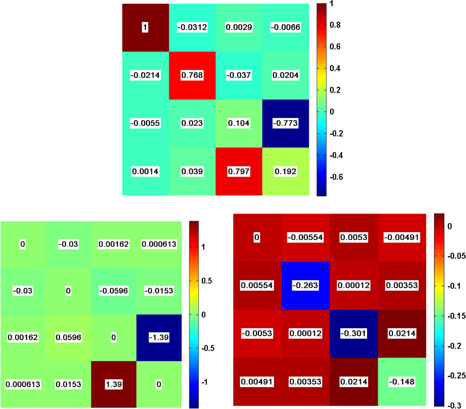oncentration of sucrose = 1 M$ , $χ = 1.96 \deg . {cm}^{- 1}$ ), turbid ( $μ_{s} = 30 {cm}^{- 1}$ , $g = 0.95$ ) phantom.

Table 2

The values for the polarization parameters extracted using Eqs. (14)–(19) (third column). The values for the parameters extracted via retarder polar decomposition using Eqs. (2)–(7) for sequential linear retardance and optical rotation effects. The R, δ and Ψ- parameters extracted using Eqs. (23)–(25), for simultaneous δ and Ψ effects (fifth column). The uncertainty of the parameter Ψlog-M was very small ∼10−5) and hence not given. The first column shows the control inputs. The control input for the net depolarization coefficient Δ was determined from the experimental Mueller matrix of the pure depolarizing phantom having no birefringence and optical activity. The expected value for linear retardance (δ) and optical rotation (Ψ) are estimated by using the corresponding values from the nonscattering phantom (δ0 and Ψ0) and accounting for increased pathlength [δ=δ0×〈L〉, Ψ=Ψ0×〈L〉, 〈L〉=1.17 cm MC-derived average photon pathlength).

Parameters	Control input	Differential matrix	Retarder polar decomposition (Sequential)	Retarder polar decomposition (Simultaneous)
$Δ$	$\sim 0.188$	0.211	0.210	0.210
$δ$ (radian)	$\sim 1.574$	$1.386 \pm 0.022$	1.384	1.386
$Ψ$ (radian)	$\sim 0.030$	0.030	0.036	0.030
R (radian)	$\sim 1.575$	1.387	1.387	1.387
$D$	$\sim 0$	$0.030 \pm 0.009$	0.032	0.032

In Fig. 3, we show the Monte Carlo simulation-generated Mueller matrix and the corresponding $L_{m}$ and $L_{u}$ matrices for a birefringent (anisotropy in refractive index $Δ n = 1.36 \times 10^{- 5}$ , that corresponds to a value of $δ = 1.34 rad$ for a path length of 1 cm), chiral (optical activity $χ = 1.96 \deg . {cm}^{- 1}$ ), turbid medium ( $μ_{s} = 60 {cm}^{- 1}$ , $g = 0.95$ , $thickness = 1 cm$ ), in the backward detection geometry. The results are shown for scattered light collected at a spatial position 3 mm away from the point of illumination in the backscattering geometry. The determined values for the polarization parameters are listed in Table 3. Once again, the depolarization coefficients ( $Δ$ ) derived from both the formalisms agree reasonably well. The slightly larger value for the diattenuation $D$ (extracted from both formalisms) in the backscattering geometry as compared to forward scattering geometry is attributed to the scattering-induced diattenuation effect (which primarily arises due to the contribution of singly/weakly backscattered photons).²⁶ Since this backscattering-induced diattenuation effect is not exhibited in a completely distributed fashion, the resulting diattenuation parameter extracted from the differential matrix deviates slightly from that extracted from the polar decomposition. Further, since the effect of the curved-propagation path is more pronounced in the backscattering geometry, the resulting reduction in the apparent linear retardance is also more prominent in the backscattering geometry as compared to forward scattering geometry.²⁶ The reduction of net optical rotation (in contrast to forward scattering geometry) is also known to originate from the contribution of the backscattered photons (that suffer scattering in the backward hemisphere only) which changes the handedness of rotation, leading to cancelation of net optical rotation.²⁶ As observed before, use of retarder polar decomposition leads to systematic underestimation of the value of $Ψ$ . Never-the-less, this discrepancy is resolved when these are determined using Eqs. (24) and (25), for simultaneously occurring $δ$ and $Ψ$ effects. Further, the differential matrix-derived uncertainty in linear retardance ( $Δ δ^{\log - M}$ ) is observed to be higher in the backscattering geometry as compared to the forward scattering geometry. The stronger random orientation effects of linear birefringence (as observed in the photon’s reference frame) and enhanced depolarization effects in the backscattering geometry account for the larger uncertainty in linear retardance. Similarly, contribution of optical rotation of different handedness from two distinct subgroups of photons (photons that undergo a series of forward scattering events to eventually emerge in the backward direction, and the back-scattered photons) might lead to the observed slightly nonzero value for uncertainty of net optical rotation ( $Δ Ψ^{\log - M}$ ).

Fig. 3

Top: The Monte Carlo simulation-generated Mueller matrix and the corresponding $L_{m}$ and $l_{u}$ matrices for a birefringent (anisotropy in refractive index $Δ n = 1.36 \times 10^{- 5}$ , that corresponds to a value of $δ = 1.34$ radian for a path length of 1 cm), chiral (optical activity $χ = 1.96 \deg . {cm}^{- 1}$ ), turbid medium ( $μ_{s} = 60 {cm}^{- 1}$ , $g = 0.95$ , $thickness = 1 cm$ ), in the backward detection geometry. The results are shown for scattered light collected at a spatial position 3 mm away from the point of illumination in the backscattering geometry.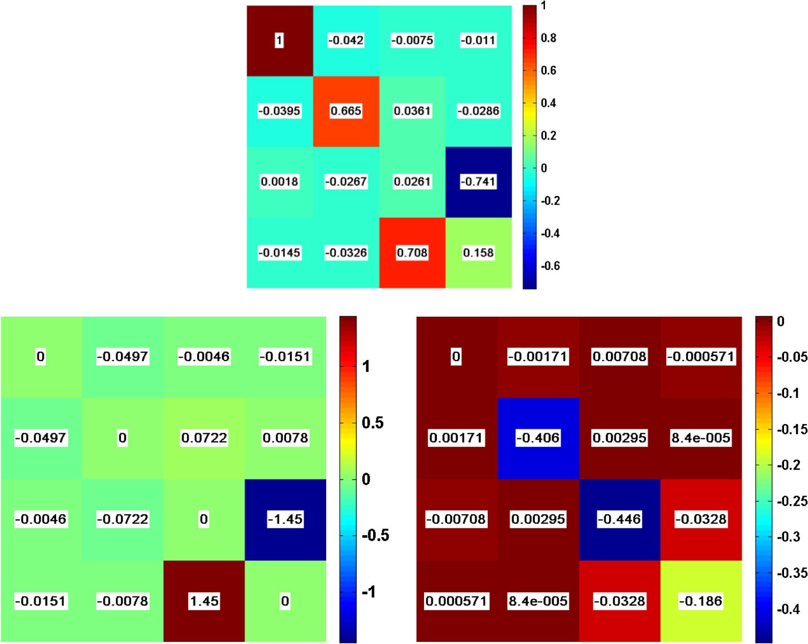

Table 3

The values for the polarization parameters extracted using Eqs. (14)–(19) (third column). The values for the parameters extracted via retarder polar decomposition using Eqs. (2)–(7) for sequential linear retardance and optical rotation effects. The R, δ and Ψ -parameters extracted using Eqs. (23)–(25), for simultaneous δ and Ψ effects (5th column). The first column shows the control inputs. The control input for the net depolarization coefficient Δ was determined from the MC-generated Mueller matrix of the pure depolarizing phantom having no birefringence and optical activity. The expected value for linear retardance (δ) and optical rotation (Ψ) are estimated by using the intrinsic Δn and χ values and accounting for increased pathlength [δ=(2π/λ)Δn×〈L〉, Ψ=χ×〈L〉, 〈L〉=1.33 cm MC-derived average pathlength).

Parameters	Control input	Differential matrix	Retarder polar decomposition (Sequential)	Retarder polar decomposition (Simultaneous)
$Δ$	$\sim 0.28$	0.293	0.290	0.290
$δ$ (radian)	$\sim 1.782$	$1.45 \pm 0.033$	1.444	1.444
$Ψ$ (radian)	$\sim 0.046$	$0.036 \pm 0.003$	0.044	0.036
R (radian)	$\sim 1.784$	1.452	1.446	1.446
$D$	$\sim 0$	$0.052 \pm 0.007$	0.044	0.044

In order to further test the validity of the retarder polar decomposition for simultaneous effects (Eqs. (24) and (25) of Sec. 2.4), for the extraction of $δ$ and $Ψ$ -parameters from media exhibiting these effects simultaneously, in the following we present the decomposition results of Mueller matrices from a liquid crystal-based twisted nematic spatial light modulator (TNSLM, LC-R 2500, Holoeye Photonics, Germany) in transmission geometry. TNSLM is an optical element whereby the linear retardance and optical rotation effects can be assumed to be occurring simultaneously over the thickness of the liquid crystal layer.²⁷^,²⁸ The linear retardance effect arises due to the orientation of the liquid crystal molecules whereas the optical rotation arises owing to the molecular twist over the thickness of the liquid crystal layers.²⁸ Figure 4(a) and 4(b) shows the variation of the derived $δ$ and $Ψ$ -parameters respectively, as a function of varying gray level (address voltage) of the TNSLM. One can observe that with decreasing gray levels (increasing the address voltage), both $δ$ and $Ψ$ -parameters approach zero. This occurs because, with increasing address voltage, the bulk liquid crystal directors tend to get aligned along the electric field direction, resulting in reduction of both $δ$ and $Ψ$ -parameters.²⁷^,²⁸ In agreement with previous reports,²⁷ at higher gray levels (close to the maximum value 255), the value for $Ψ$ reaches its maximum and the value for $δ$ initially increases and then shows a decreasing trend. In general, the Mueller matrices of the TNSLM exhibited very low depolarization values (not shown), possibly arising due to orientation fluctuations of the molecules. Importantly, $δ$ and $ψ$ -parameters derived via differential matrix formalism and retarder polar decomposition with its associated algebra [Eqs. (5) and (6)] for sequential occurrence of linear retardance and optical rotation, show significant discrepancy. It is apparent that retarder polar decomposition [Eq. 4)] leads to systematic underestimation of $δ$ and overestimation of the value for $Ψ$ . While the overestimation effect of the $Ψ$ -parameter was also noticed for the optical phantoms, the underestimation effect of $δ$ -parameter becomes more apparent here. This is because of the considerably higher magnitude of the optical rotation for the TNSLM as compared to that of the optical phantoms. As can be noticed, the retarder polar decomposition for simultaneous linear retardance and optical rotation effects [Eqs. (24) and (25)], results in complete agreement of the derived $δ$ and $Ψ$ -parameters with the differential matrix formalism.

Fig. 4

Comparison of the extracted values of ( $a$ ) linear retardance $δ$ and ( $b$ ) optical rotation $Ψ$ obtained from the differential matrix decomposition (Eqs. (14), (15), shown by solid circles), the derived values, respectively obtained from retarder polar decomposition using Eqs. (5) and (6) which assumes sequential occurrence of linear retardance and optical rotation effects (triangles) and Eqs. (24) and (25) for simultaneous linear retardance and optical rotation effects (squares) as a function of increasing gray level of the TNSLM in transmission mode.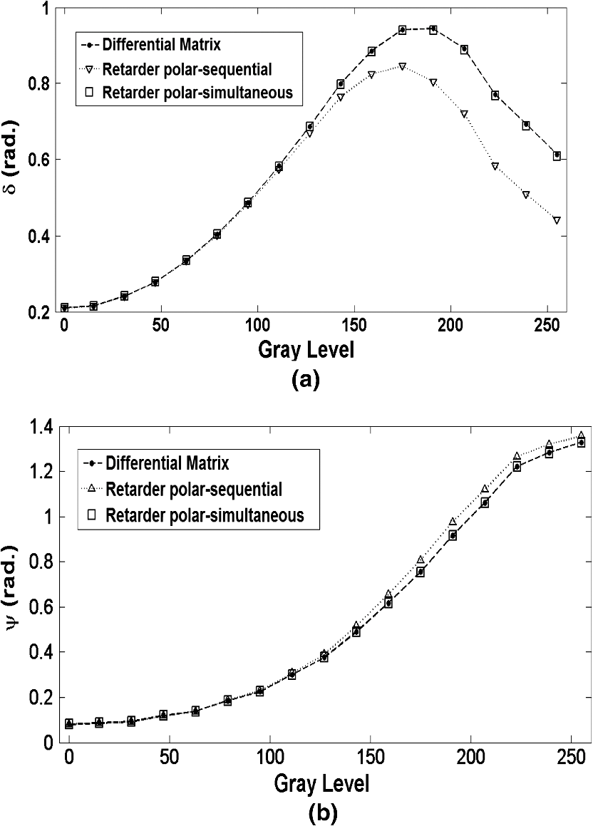

The results presented above clearly demonstrate that the intrinsic polarization parameters (specifically, $δ$ and $Ψ$ and $Δ$ ) of a medium exhibiting simultaneous polarization effects, can be ‘self-consistently’ extracted from both the differential matrix and the polar decomposition approach corrected for simultaneous occurrence of linear retardance and optical rotation effects. Moreover, the results on the tissue phantoms indicate that the differential matrix formalism yields additional polarization metrics on the uncertainty of the polarization parameters (specifically, $Δ δ^{\log - M}$ of linear retardance), which can be of potential use for probing local organization (disorganization) of birefringent tissue structures. We have thus explored such possibility in the context to monitoring of myocardial tissue regeneration following stem cell therapy (through quantification of linear retardance from the measured Mueller matrices), as presented below.

The Mueller matrix images from myocardial tissue samples from Lewis rat, both with and without stem-cell treatment, were recorded using our imaging polarimetry system. In agreement with our previous results on the use of our point polarimetry system,²³^,²⁴ the results showed a large decrease in the magnitude of linear retardance ( $δ$ ) in the infarcted region of the untreated myocardium. In contrast, in the infarcted region after stem-cell treatment, an increase of $δ$ towards native levels was observed (images not shown here), indicating re-growth and re-organization of the myocardium. Moreover, the differential matrix-derived polarimetry images showed interesting spatial behavior, as shown in Fig. 5(a), 5(b), 5(c), and 5(d). Comparison of ( $a$ ) linear retardance $δ^{\log - M}$ and ( $b$ ) depolarization $Δ^{\log - M}$ – images show certain common features. Both show considerable spatial variation. Most of the regions associated with high depolarization exhibit higher retardance values also. Note that regions exhibiting higher depolarization are possibly associated with increased photon pathlength (due to increased ventricular thickness with stem-cell treatment²⁴), and thus consequently exhibit higher linear retardance values. Never-the-less, many of the features in the linear retardance image may be attributed to the intrinsic variation of birefringence also. The orientation angle of birefringence $θ^{\log - M}$ –image ( $c$ ), derived via Eq. (15), also shows interesting spatial variation. In general, the spatial variations of $θ^{\log - M}$ are more prominent towards the edges, whereas in the middle region these are weaker (i.e., show better uniformity). The variations through the myocardial wall are likely due to the change in orientation of the myocyte fibers through the wall. The orientation of the fibers undergoes a rotation from the outside of the ventricle to the inside, leading to a rapid change in orientation angle towards the edges.²⁴ In contrast, near the center of the ventricular wall the fibers are nearly uniformly aligned. It is interesting to note that the derived uncertainty of linear retardance ${Δ δ}^{\log - M}$ —image ( $d$ ) exhibits some kind of correlated behavior with the $θ^{\log - M}$ —image ( $c$ ). Regions with larger variation of orientation angle $θ^{\log - M}$ are observed to exhibit larger uncertainty in the derived linear retardance ( ${Δ δ}^{\log - M}$ ). This is expected because rapid local changes in orientation angle of birefringence should in general lead to larger uncertainty in linear retardance derived via the differential matrix decomposition (from $L_{u}$ matrix). Moreover, such local changes in orientation angle of birefringence should also lead to additional depolarization effects. This follows because addition of the individual retardance matrices having random orientation of axes manifests as depolarization.⁴ This is likely to be the case observed here [Fig. 5(b)]. Thus, it appears that the differential matrix decomposition-derived parameters, $Δ^{\log - M}$ , $δ^{\log - M}$ , $θ^{\log - M}$ , and $Δ δ^{\log - M}$ provide complementary and useful information on the morphology of the tissue: overall scattering properties via $Δ^{\log - M}$ , anisotropic organization of tissue structures via $δ^{\log - M}$ , local organization (or disorganization) of birefringent tissue structures via $θ^{\log - M}$ and $Δ δ^{\log - M}$ . These polarimetry parameters thus hold promise as useful biological metrics for quantitative polarimetric tissue characterization/diagnosis/monitoring treatment response.

Fig. 5

The differential matrix-derived (a) linear retardance $δ^{\log - M}$ (in deg), (b) net depolarization $Δ^{\log - M}$ ( $scaled \times 100$ ), (c) orientation angle of birefringence $θ^{\log - M}$ (in degrees) and (d) uncertainty of linear retardance ${Δ δ}^{\log - M}$ (in deg) images from transmission polarization measurements in 1-mm-thick sections from Lewis rat heart tissue following stem-cell treatments.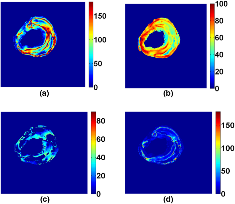

5. Conclusions

To conclude, we have performed a detailed comparative evaluation of the polar decomposition and the differential matrix decomposition of Mueller matrices for extraction/quantification of the individual, intrinsic polarimetry characteristics (with special emphasis on linear retardance $δ$ , optical rotation $Ψ$ and depolarization $Δ$ parameters) from complex tissue-like turbid media exhibiting simultaneous scattering and polarization effects. The results suggest that for media exhibiting simultaneous polarization effects, the use of retarder polar decomposition and its associated analysis (which assumes preferred sequential occurrence of linear retardance and optical rotation effects) results in systematic underestimation of $δ$ and overestimation of $Ψ$ parameters. Complete agreement between the derived $δ$ and $Ψ$ parameters from differential matrix formalism and retarder polar decomposition was obtained when the simultaneous occurrence of linear retardance and optical rotation was incorporated in the latter formalism. The self-consistency of both the decompositions was validated on the experimental and the MC-generated Mueller matrices for media exhibiting simultaneous polarization effects (linear retardance, optical rotation and depolarization). It should be noted for completeness that the influence of the remaining polarization parameter, diattenuation, on the polar decomposition and the differential matrix decomposition has recently been reported.²⁹ Since the magnitude of diattenuation is typically very weak in most tissues,¹⁴ it has not been investigated in details here. We have instead paid attention on linear retardance, optical rotation and depolarization parameters, because these three are the most prominent tissue polarimetry effects, which also hold promise as useful biological metrics. Never-the-less, the initial exploration of the differential Mueller matrix formalism for monitoring of myocardial tissue regeneration following stem cell therapy, showed that this formalism yields additional polarization metrics, and combined usage of these multiple polarimetry parameters hold promise for quantitative polarimetric tissue characterization/diagnosis. In general, the extended formulation, which is capable of tackling either the simultaneous or sequential occurrences of polarization events, might turn out to be a useful approach, particularly for the characterization of biological tissue, where no unique order (or sequence) can be assigned to the polarimetry effects.

Acknowledgments

This work was supported by Indian Institute of Science Education and Research (IISER)-Kolkata, an autonomous teaching and research institute funded by the Ministry of Human Resource Development (MHRD), Govt. of India.

References

1.

D. S. KligerJ. W. LewisC. E. Randall, Polarized Light in Optics and Spectroscopy, Academic Press–Harcourt Brace JovanovichNew York,1990). Google Scholar

2.

R. A. Chipman, “Polarimetry,” Handbook of Optics, 22.1 –22.37 2nd ed.McGraw-Hill, New York (1994). Google Scholar

3.

W. S. BickelW. M. Bailey, “Stokes vectors, Mueller matrices, and polarization of scattered light,” Am. J. Phys., 53 (5), 468 –478 (1985). http://dx.doi.org/10.1119/1.14202 AJPIAS 0002-9505 Google Scholar

4.

N. GhoshI. A. Vitkin, “Tissue polarimetry: concepts, challenges, applications and outlook,” J. Biomed. Opt., 16 (11), 110801 (2011). http://dx.doi.org/10.1117/1.3652896 JBOPFO 1083-3668 Google Scholar

5.

V. V. TuchinL. WangD. À. Zimnyakov, Optical Polarization in Biomedical Applications, Springer-Verlag, Berlin, Heidelberg, NY (2006). Google Scholar

6.

S. Manhaset al., “Mueller matrix approach for determination of optical rotation in chiral turbid media in backscattering geometry,” Opt. Express, 14 (1), 190 –202 (2006). http://dx.doi.org/10.1364/OPEX.14.000190 OPEXFF 1094-4087 Google Scholar

7.

P. J. WuJ. T. Walsh Jr., “Stokes polarimetry imaging of rat tail tissue in a turbid medium: degree of linear polarization image maps using incident linearly polarized light,” J. Biomed. Opt., 11 (1), 014031 (2006). http://dx.doi.org/10.1117/1.2162851 JBOPFO 1083-3668 Google Scholar

8.

N. GhoshM. WoodA. Vitkin, “Polarized light assessment of complex turbid media such as biological tissues using Mueller matrix decomposition,” Handbook of Photonics for Biomedical Science, 253 –282 CRC Press, Taylor & Francis Group, London (2010). Google Scholar

9.

M. F. G. Woodet al., “Towards noninvasive glucose sensing using polarization analysis of multiply scattered light,” Handbook of Optical Sensing of Glucose in Biological Fluids and Tissues, CRC Press, Taylor & Francis Group, London (2009). Google Scholar

10.

S. Yau LuR. A. Chipman, “Interpretation of Mueller matrices based on polar decomposition,” J. Opt. Soc. Am. A, 13 (5), 1106 –1113 (1996). http://dx.doi.org/10.1364/JOSAA.13.001106 JOAOD6 0740-3232 Google Scholar

11.

R. OssikovskiA. De MartinoS. Guyot, “Forward and reverse product decompositions of depolarizing Mueller matrices,” Opt. Lett., 32 (6), 689 –691 (2007). http://dx.doi.org/10.1364/OL.32.000689 OPLEDP 0146-9592 Google Scholar

12.

R. Ossikovski, “Analysis of depolarizing Mueller matrices through a symmetric decomposition,” J. Opt. Soc. Am. A, 26 (5), 1109 –1118 (2009). http://dx.doi.org/10.1364/JOSAA.26.001109 JOAOD6 0740-3232 Google Scholar

13.

R. Ossikovskiet al., “Depolarizing Mueller matrices: how to decompose them?,” Phys. Stat. Sol. (a)., 205 (4), 720 –727 (2008). http://dx.doi.org/10.1002/pssa.200777793 Google Scholar

14.

N. GhoshM. F. G. WoodI. A. Vitkin, “Influence of the order of the constituent basis matrices on the Mueller matrix decomposition-derived polarization parameters in complex turbid media such as biological tissues,” Opt. Commun., 283 (6), 1200 –1208 (2010). http://dx.doi.org/10.1016/j.optcom.2009.10.111 OPCOB8 0030-4018 Google Scholar

15.

R. Ossikovski, “Differential matrix formalism for depolarizing anisotropic media,” Opt. Lett., 36 (12), 2330 –2332 (2011). http://dx.doi.org/10.1364/OL.36.002330 OPLEDP 0146-9592 Google Scholar

16.

N. Ortega-QuijanoJ. L. Arce-Diego, “Mueller matrix differential decomposition,” Opt. Lett., 36 (10), 1942 –1944 (2011). http://dx.doi.org/10.1364/OL.36.001942 OPLEDP 0146-9592 Google Scholar

17.

R. C. Jones, “New calculus for the treatment of optical systems. VII. Properties of the

N

-matrices,” J. Opt. Soc. Am., 38 (8), 671 –683 (1948). http://dx.doi.org/10.1364/JOSA.38.000671 JOSAAH 0030-3941 Google Scholar

18.

R. M. A. Azzam, “Propagation of partially polarized light through anisotropic media with or without depolarization: a differential

4 \times 4

matrix calculus,” J. Opt. Soc. Am., 68 (12), 1756 –1767 (1978). http://dx.doi.org/10.1364/JOSA.68.001756 JOSAAH 0030-3941 Google Scholar

19.

N. GhoshM. F. G. WoodI. A. Vitkin, “Mueller matrix decomposition for extraction of individual polarization parameters from complex turbid media exhibiting multiple scattering, optical activity and linear birefringence,” J. Biomed. Opt., 13 (4), 044036 (2008). http://dx.doi.org/10.1117/1.2960934 JBOPFO 1083-3668 Google Scholar

20.

R. Ossikovski, “Differential and product Mueller matrix decompositions: a formal comparison,” Opt. Lett., 37 (2), 220 –222 (2012). http://dx.doi.org/10.1364/OL.37.000220 OPLEDP 0146-9592 Google Scholar

21.

H. D. NobleR. A. Chipman, “Mueller matrix roots algorithm and computational considerations,” Opt. Express, 20 (1), 17 –31 (2012). http://dx.doi.org/10.1364/OE.20.000017 OPEXFF 1094-4087 Google Scholar

22.

O. ArteagaA. Canillas, “Psuedopolar decomposition of the Jones and Mueller-Jones exponential polarization matrices,” J. Opt. Soc. Am. A, 26 (4), 783 –793 (2009). http://dx.doi.org/10.1364/JOSAA.26.000783 JOAOD6 0740-3232 Google Scholar

23.

N. Ghoshet al., “Mueller matrix decomposition for polarized light assessment of biological tissues,” J. Biophotonics, 2 (3), 145 –156 (2009). http://dx.doi.org/10.1002/jbio.v2:3 1864-0648 Google Scholar

24.

M. F. G. Wood, “Polarization birefringence measurements for characterizing the myocardium, including healthy, infracted, and stem cell treated regenerating cardiac tissues,” J. Biomed. Opt., 15 (4), 047009 (2010). http://dx.doi.org/10.1117/1.3469844 JBOPFO 1083-3668 Google Scholar

25.

M. F. G. WoodX. GuoI. A. Vitkin, “Polarized light propagation in multiply scattering media exhibiting both linear birefringence and optical activity: Monte Carlo model and experimental methodology,” J. Biomed. Opt., 12 (1), 014029 (2007). http://dx.doi.org/10.1117/1.2434980 JBOPFO 1083-3668 Google Scholar

26.

N. GhoshM. F. G. WoodI. A. Vitkin, “Polarimetry in turbid, birefringent, optically active media: a Monte Carlo study of Mueller matrix decomposition in the backscattering geometry,” J. Appl. Phys., 105 (10), 102023 (2009). http://dx.doi.org/10.1063/1.3116129 JAPIAU 0021-8979 Google Scholar

27.

V. DuránJ. LancisE. TajahuerceM. Fernández-Alonso, “Phase-only modulation with a twisted nematic liquid crystal display by means of equi-azimuth polarization states,” Opt. Express, 14 (12), 5607 –5616 (2006). http://dx.doi.org/10.1364/OE.14.005607 OPEXFF 1094-4087 Google Scholar

28.

J. L. de Bougrenet de la TocnayeL. Dupont, “Complex amplitude modulation by use of liquid-crystal spatial light modulators,” Appl. Opt., 36 (8), 1730 –1741 (1997). http://dx.doi.org/10.1364/AO.36.001730 APOPAI 0003-6935 Google Scholar

29.

N. Ortega-Quijanoet al., “Experimental validation of Mueller matrix differential decomposition,” Opt. Express, 20 (2), 1151 –1163 (2012). http://dx.doi.org/10.1364/OE.20.001151 OPEXFF 1094-4087 Google Scholar

Citation Download Citation

Satish Kumar, Harsh Purwar, Razvigor Ossikovski, I. Alex Vitkin, and Nirmalya Ghosh "Comparative study of differential matrix and extended polar decomposition formalisms for polarimetric characterization of complex tissue-like turbid media," Journal of Biomedical Optics 17(10), 105006 (12 October 2012). https://doi.org/10.1117/1.JBO.17.10.105006

Published: 12 October 2012

Access the abstract

JOURNAL ARTICLE
12 PAGES

DOWNLOAD PAPER SAVE TO MY LIBRARY

GET CITATION

CITATIONS

Cited by 56 scholarly publications and 1 patent.

Explore citations on Lens.org

RIGHTS & PERMISSIONS

Get copyright permission Get copyright permission on Copyright Marketplace

KEYWORDS

Polarization

Polarimetry

Tissues

Wave plates

Mueller matrices

Tissue optics

Birefringence

1.

Introduction

2.

Theory

2.1.

Polar Decomposition of Mueller Matrix

Eq. (1)

Eq. (2)

Eq. (3)

Eq. (4)

Eq. (5)

Eq. (6)

Eq. (7)

2.2.

Differential Matrix Decomposition

Eq. (8)

Eq. (9)

Eq. (10)

Eq. (11)

Eq. (12)

Eq. (13)

Eq. (14)

Eq. (15)

Eq. (16)

Eq. (17)

2.3.

Conversion Relations for the Polarization Parameters

Eq. (18)

Eq. (19)

2.4.

Analytical Extension for “Self-Consistent” Extraction of Linear Retardance δ and Optical Rotation Ψ

Eq. (20)

Eq. (21)

Eq. (22)

Eq. (23)

Eq. (24)

Eq. (25)

Eq. (26)

Eq. (27)

3.

Experimental Methods

3.1.

Experimental Polarimetry Systems

Eq. (28)

Eq. (29)

3.2.

Forward Polarization Sensitive Monte Carlo Simulation Model

4.

Results and Discussion

Fig. 1

Table 1

Fig. 2

Table 2

Fig. 3

Table 3

Fig. 4

Fig. 5

5.

Conclusions

Acknowledgments

References

Show All Keywords

Keywords/Phrases

Search In:

Publication Years

Analytical Extension for “Self-Consistent” Extraction of Linear Retardance $δ$ and Optical Rotation $Ψ$