Detection of cerebral autoregulation by near-infrared spectroscopy in neonates: performance analysis of measurement methods

Alexander Caicedo; Gunnar Naulaers; Petra Lemmers; Frank van Bel; Martin Wolf; Sabine Van Huffel

doi:10.1117/1.JBO.17.11.117003

1 November 2012 Detection of cerebral autoregulation by near-infrared spectroscopy in neonates: performance analysis of measurement methods

Alexander Caicedo, Gunnar Naulaers, Petra Lemmers, Frank van Bel, Martin Wolf, Sabine Van Huffel

Author Affiliations +

Journal of Biomedical Optics, Vol. 17, Issue 11, 117003 (November 2012). https://doi.org/10.1117/1.JBO.17.11.117003

Abstract

Cerebral Autoregulation, in clinical practice, is assessed by means of correlation or coherence analysis between mean arterial blood pressure (MABP) and cerebral blood flow (CBF). However, even though there is evidence linking cerebral autoregulation assessment with clinical outcome in preterm infants, available methods lack precision for clinical use. Classical methods, used for cerebral autoregulation, are influenced by the choice of parameters such as the length of the epoch under analysis and the choice of suitable frequency bands. The influence of these parameters, in the derived measurements for cerebral autoregulation, has not yet been evaluated. In this study, cerebral autoregulation was assessed using correlation, coherence, a modified version of coherence and transfer function gain, and phase. The influence of the extra-parameters on the final scores was evaluated by means of sensitivity analysis. The methods were applied to a database of 18 neonates with measurements of MABP and tissue oxygenation index (TOI). TOI reflects changes in CBF and was measured by means of near-infrared spectroscopy.

1. Introduction

Cerebral autoregulation is a mechanism used by the brain in order to maintain a constant cerebral blood flow (CBF) in the presence of changes in mean arterial blood pressure (MABP). This mechanism was first described in humans by Lassen.¹ Studies of cerebral autoregulation have aimed to measure the coupling between MABP and CBF by means of linear and nonlinear techniques.²^,³ Linear techniques were mostly studied; however, their clinical use is still restricted.² Some studies of cerebral autoregulation in neonates point out a correlation between impaired cerebral autoregulation and clinical outcome, however, available methods lack of precision for its clinical use.⁴^,⁵

There are several limitations to the use of cerebral autoregulation assessment in clinical practice. Reliable measurements of CBF are hard to obtain. Methods using ultrasound Doppler may produce variations in physiological parameters when used over longer periods of time, however, they are also highly sensitive to movement artifacts.⁶ Moreover, the lack of a gold standard in cerebral autoregulation complicates the validation of the methods used for its assessment. Near-infrared spectroscopy (NIRS) represents an attractive method for the noninvasive assessment of CBF and cerebral autoregulation. In these studies, cerebral oxygenation parameters are used as a parameter for CBF and mean arterial blood pressure (MABP) as a parameter of the cerebral perfusion pressure. With the classic near-infrared studies, using the Beer-Lambert law, oxygenated ( ${HbO}_{2}$ ) and deoxygenated hemoglobin (HbR) can be measured. Different studies showed a good correlation between HbD ( $HbD = {HbO}_{2} - HbR$ ) and CBF.⁷ Tsjui et al. first described the coherence between HbD and MABP as a measure of cerebral autoregulation, provided that the oxygen saturation remained stable.⁸ A higher incidence of intraventricular bleedings was described in a group of premature infants when the coherence was more than 0.5. This group also described the Passive Pressure Index (PPI) as the percentage of time that a coherence of more than 0.77 was found between MABP and HbD, using transfer function analysis between the 0 and 0.04 Hz frequency band.⁴ A significant correlation was found between the PPI and intraventricular bleedings in premature infants.⁹ However, HbD remains a difficult parameter to measure continuously in a neonatal intensive care unit and, therefore, newer parameters measured with spatially resolved spectroscopy such as the tissue oxygenation index (TOI) and the regional oxygen saturation ( ${rSO}_{2}$ ) are used.¹⁰ TOI is calculated by $[{HbO}_{2} / ({HbO}_{2} + HbR)] * 100 (%)$ and represents the percentage of oxygenated hemoglobin present in the tissue. These parameters are absolute values and reflect the cerebral oxygenation. Recently, we demonstrated that TOI and ${rSO}_{2}$ can be used instead of HbD to measure cerebral autoregulation.¹¹ Wong et al. showed that changes in tissue oxygenation index (TOI), measured by means of NIRO 300 (Hamamatsu, Japan), correlate with changes in CBF in frequencies below 0.1 Hz.¹²

Considering this, NIRS represents an attractive method for the noninvasive assessment of CBF and cerebral autoregulation.¹³ Recently, the interest for the use of NIRS in the study of cerebral autoregulation has been increased.⁴^,⁵^,¹⁴^,¹⁵ Wong et al. found a higher gain between MABP and TOI in the group of premature infants that was younger (PMA of 24 weeks) and had a higher mortality and incidence in serious intraventricular bleedings.⁵ Hahn et al. found a good correlation between the gain (in the group where the coherence was more than 0.5 between MABP and TOI) measured with NIRS and the autoregulatory capacity measured with Doppler flow in piglets.¹⁶

Correlation has been used in order to quantify the strength of the relation between MABP and CBF after head injury.¹⁷ The first one using transfer function analysis for autoregulation assessment was Giller.¹⁸ Giller showed that patients with impaired autoregulation presented higher coherence coefficients. Coherence, as well as transfer function analysis, is a frequency based method. Transfer function analysis is based on the system identification framework where the system, in this case the mechanisms involved in cerebral autoregulation, is treated as a black box and the frequency response is calculated based on measurements of the input and the output, MABP and CBF, respectively.¹⁹ Coherence and transfer function analysis have also been used with NIRS signals in order to assess cerebral autoregulation.⁴^,⁵ The core of transfer function analysis, and frequency based techniques, is the estimation of the power spectral and cross-spectral densities of the input and the output. This estimation is normally done using the Welch method.²⁰ This method takes advantage of the stationarity of a signal in order to reduce the influence of the noise, the bias, and the variance in the spectrum estimation. However, if the signal presents nonstationarities, the estimation is biased. In addition, extra parameters are needed in order to estimate the power spectra, however, an arbitrary choice of these parameters can produce misleading results. In the literature, there is a lack of studies that investigate the influence of the selection of those parameters when used for cerebral autoregulation assessment. In addition, there is no consensus on which parameters to use and it is common to find different choices in different studies. Therefore, in this study, we aimed to investigate the influence of the change in these parameters on the final scores used for autoregulation assessment. Additionally, we aim to identify which method is more robust against changes on these parameters, as well as the values to be selected when using correlation, coherence or transfer function for cerebral autoregulation assessment.

2. Data

This study is based on measurements from 18 infants, with need for intensive care, that were monitored during the first days of life at the neonatal intensive care unit (NICU) of the University hospital Leuven (Belgium). ${SaO}_{2}$ was measured continuously by pulse oximetry at the right hand in all the patients. MABP was monitored continuously by an indwelling umbilical arterial catheter. Transcranial NIRS was used for noninvasive monitoring of cerebral hemodynamics and oxygenation. A NIRO300 instrument was used for the continuous recording of TOI (Hamamatsu®, Japan). The neonates had a mean post menstrual age (PMA) of 27.9 weeks (25.9 to 29.2 weeks), a mean body weight of 991 g (728.5 to 1231.5 g) and the mean recording time was 3h54m (2h24m–4h8m). MABP and ${SaO}_{2}$ were analog and digitized afterwards by the CODAS system (Dataq Instruments, USA). The NIRO 300 optodes were placed at the right frontoparietal side of the infant, with a 4-cm interoptode distance, and the signals were acquired with a sampling rate of 6 Hz. They were converted to analog signals with a sample-and-hold function before being introduced in the CODAS system. The differential path length (taking into account the scattering of the near-infrared light into the brain) was set at 4.39 and encoded into the personal computer as a constant value.¹⁶^,²¹

The signals were filtered using a low-pass and a high-pass filter with cut-off frequencies of 0.15 and 0.003 Hz, respectively. The data was downsampled, afterward, to a sampling frequency $Fs = 0.3 Hz$ . As the information we are interested in is located in frequencies lower than 0.1 Hz, this cut-off frequency does not affect the frequency range of which we are interested. Artifacts, such as movements and changes in baseline, were detected and removed by an algorithm implemented in Matlab. This algorithm trained a least squares support vector machine (LS-SVM) to interpolated data whenever the duration of the artifact was shorter than 30 s, else the signal was truncated.²² Hence, a continuous recording was divided in smaller segments which were free of artifacts and only segments with lengths longer than 40 min were kept for further analysis. Remaining artifacts, which could not be detected in the previous step, were deleted manually. Figure 1 shows the data from one measurement segment for one patient, the scores from correlation, coherence, and gain. The coherence and gain values were averaged in three different frequency bands which were 0.003 to 0.02 Hz very low frequency (VLF), 0.02 to 0.05 Hz low frequency (LF), and 0.05 to 0.1 Hz high frequency (HF).

Fig. 1

Correlation, coherence and gain values for measurements from one patient. In the upper figure the raw data: MABP and TOI. In the second figure the correlation values; the signal was divided in overlapping epochs of 15 min long and with a 90% overlapping. The third figure presents the coherence values averaged in three different frequency bands VLF (0.003 to 0.02 Hz), LF (0.02 to 0.05 Hz) and HF (0.05 to 0.1 Hz), the signal was divided in epochs of 15 min long, a subwindow length of 5 min was used in the Welch method with an overlapping percentage of 90%. The last figure shows the gain values for the same parameter setup as for the coherence.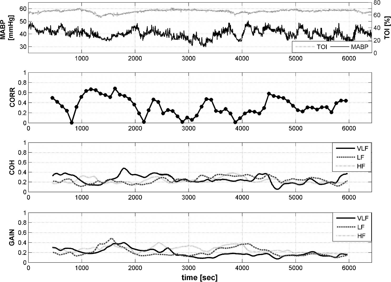

3. Methods

Cerebral autoregulation was assessed using four different methods which include correlation, coherence, modified coherence, and transfer function. The influence of the epoch length, overlapping percentage, and subwindow length on the final scores was evaluated. From here on, the term epochs refers to the segment on which the scores are calculated, the term subwindows refers to the segment used in the Welch method. The overlapping percentage refers to different parameters in the correlation and the frequency based methods and it will be further explained when needed.

3.1.

Correlation

Correlation (CORR) is a statistical measurement of the linear dependences between two signals. The most common measurement of correlation is called the Pearson correlation coefficient and it is expressed by:

Eq. (1)

ρ (x, y) = \frac{ε [(x - μ_{x}) (y - μ_{y})]}{σ_{x} σ_{y}},

where

ρ (x, y)

is the correlation coefficient,

ε []

represents the mathematical expectation operator,

μ_{x}

,

μ_{y}

,

σ_{x}

, and

σ_{y}

represent the mean value and standard deviation of

x

and

y

, respectively. Normally, the correlation coefficient

ρ

varies between

- 1

and 1, with 0 representing no correlation, 1 representing perfect positive correlation and

- 1

perfect negative correlation. For this study, the absolute value of the correlation was taken as a score for cerebral autoregulation.

To assess cerebral autoregulation using CORR, the data is divided in epochs, of which, the length is user-defined. The calculated CORR is then assigned to each epoch and the procedure is repeated until the complete signal is analyzed. Normally, there is no overlapping between consecutive epochs, however, by including an overlapping, a more detailed view of the evolution in the common dynamics of the two signals is obtained. Furthermore, in order to assess cerebral autoregulation in neonates, some extra parameters such as mean, standard deviation, among others, are derived from the time series of calculated CORR values. Since there is a delay between MABP and TOI of approximate 10 s in neonates, we have performed the analysis taking this delay into account.²³

In this study, we are interested on investigating the influence of the epoch length and the overlapping percentage, for consecutive epochs, on the resulting CORR scores. The following setup was used:

(1) The signals were segmented in consecutive overlapping epochs of length $T_{i}$ , where $T_{i}$ varies from 10 to 30 min.
(2) Overlapping percentages ( $O_{j}$ ) between consecutive epochs ranging from 10% to 90% were used.
(3) The CORR scores were calculated for each epoch of length $T_{i}$ and Overlapping $O_{j}$ .
(4) The mean value of the resulting CORR scores, for each $T_{i}$ and $O_{j}$ , was assigned to each patient.
(5) A sensitivity analysis was used to quantify the impact of $T_{i}$ and $O_{j}$ on the scores calculated in the previous step.

3.2.

Coherence

Coherence (COH) can be interpreted as the equivalent of correlation in the frequency domain. For each frequency component, the coherence gives a value that represents the strength of the relation between the signals at that particular frequency. The COH is calculated as expressed by:

Eq. (2)

C_{x y} = \frac{{| G_{x y} |}^{2}}{G_{x x} G_{y y}},

where

G_{x y}

represents the cross-spectral density between the signals

x

and

y

,

G_{x x}

and

G_{y y}

represent the auto-spectral density of

x

and

y

, respectively.

In order to estimate the cross-spectral and auto-spectral power densities, the Welch method is used.²⁰ For two signals $x$ and $y$ , this method segments the signals in consecutive overlapping subwindows ( $x_{L_{i} O_{j}}, y_{L_{i} O_{j}}$ ) of length $L_{i}$ , and overlapping percentage $O_{i}$ . For each one of these subwindows, the power spectrum is estimated as:

Eq. (3)

g_{x y} = F^{*} (x_{L_{i} O_{j}}) F (y_{L_{i} O_{j}}),

where

F

denotes the Fourier transform of the data and * denotes the complex conjugate. The cross-power spectrum between

x

and

y

is obtained as the mean value of the subwindows power spectrum.

Eq. (4)

G_{x y} = ε [g_{x y}] .

When

x

and

y

are stationary signals, this procedure reduces the bias and the variance in the estimation of

G_{x y}

, as the differences in the power spectrum for different subwindows are only attributed to noise, and its influence is reduced when averaging. Lower values of

L_{i}

and/or higher values for

O_{i}

produce more subwindows which improves the estimation of

G_{x y}

. For stationary signals, an

O_{i}

higher than 50% does not significantly reduce the bias and variance in the power spectrum estimation. In addition, the lowest value of

L_{i}

is limited by the lowest frequency component of interest in the analysis.

However, in real life applications, the signals $x$ and $y$ are recorded for several hours and are highly affected by nonstationarities. In order to reduce the influence of these nonstationarities in the power spectrum estimation, the most intuitive action is to reduce the length of the $x$ and $y$ , therefore, the signals are segmented in overlapping epochs of length $T_{i}$ . In order to have a better resolution in time for the evolution of the common dynamics between $x$ and $y$ , maximum overlapping between epochs is suggested. Furthermore, the relation between the nonstationarities and the length of the subwindows and their overlapping percentage ( $L_{i}$ , $O_{j}$ ) used in the Welch method has not been analyzed. Studies of cerebral autoregulation, using NIRS signals, are focused to the low frequency range of 0.003 to 0.1 Hz. In order to assess frequency components of 0.003 Hz, theoretically, a subwindow of 5 min in length is needed.

We are interested in studying the influence of the epoch length $T_{i}$ and the subwindow overlapping percentage $O_{j}$ on the resulting COH scores. The following setup was used:

(1) The signals were segmented in consecutive overlapping epochs of length $T_{i}$ , where $T_{i}$ varies from 10 to 30 min. Maximum overlapping between epochs was used.
(2) The subwindow length was fixed to $L_{i} = 5 \min$ .
(3) Overlapping percentages ( $O_{j}$ ) between consecutive subwindows ranging from 10% to 90% were used.
(4) The COH scores were calculated for each epoch of length $T_{i}$ and for each subwindow overlapping $O_{j}$ .
(5) The mean value of the resulting COH scores along the epochs, for each $T_{i}$ and $O_{j}$ , was assigned to each patient. This results in a vector of COH values in frequency per patient.
(6) A sensitivity analysis was used to quantify the impact of $T_{i}$ and $O_{j}$ in the scores calculated in the step 4.

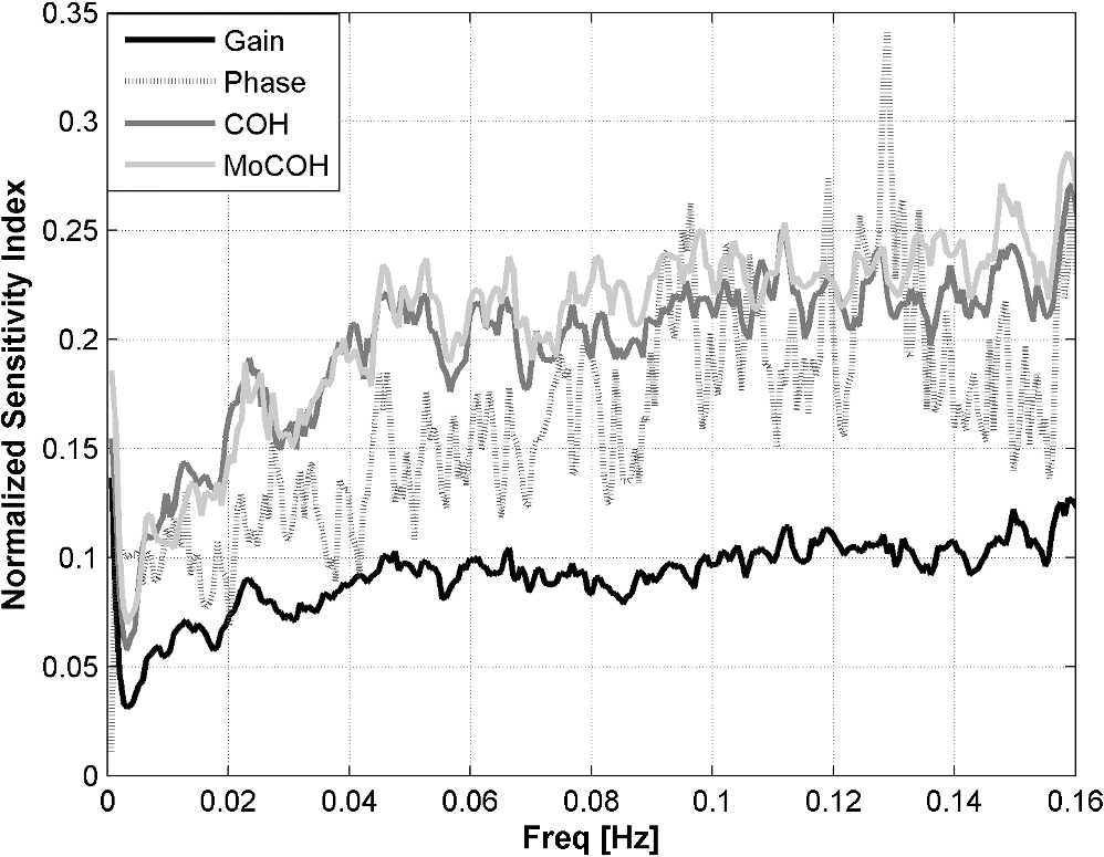
A similar setup was used for all frequency-based methods.

3.3.

Modified Coherence

As spontaneous measurements of MABP may lack enough variation needed to provide meaningful estimates of the coherence values, Hahn et al.²⁴ developed a modified version of the coherence where each frequency component of the coherence is weighted by the percentage of the MABP power presented at that frequency component.¹³^,²⁴ This modified coherence vector (MoCOH) corrects for the segments with small variations in MABP.

In order to study the influence of the epoch length $T_{i}$ and the subwindow overlapping percentage $O_{j}$ , for consecutive subwindows, the same setup as in COH was used.

3.4.

Transfer Function

The transfer function of a system is estimated by means of the cross-spectral and auto-spectral densities between the input and output signals, i.e.,

Eq. (5)

H (f) = \frac{G_{i o} (f)}{G_{i i} (f)},

where

H (f)

is the system transfer function,

G_{i o} (f)

is the input output cross-spectral density and

G_{i i} (f)

is the input auto-spectral density. As for the coherence, the cross-spectral and auto-spectral densities are estimated using the Welch method, therefore, the same restrictions of stationarity are required. The transfer function can be analyzed by its magnitude and phase. The magnitude or gain of the transfer function represents the strength of the relationship between the signals at each frequency component. The phase of the transfer function represents the phase delay at each frequency component between the signals.

The influence of the epoch length $T_{i}$ and the subwindow overlapping percentage $O_{j}$ , for consecutive subwindows, on the transfer function values, was studied using the same setup as in COH.

3.5.

Sensitivity Analysis

Two different analyses were performed to evaluate the sensitivity of each method to changes in the parameters. In both cases, a sensitivity analysis approach was followed. On one hand, a global analysis using a modified version of the elementary effects technique was used. The results given by this technique will indicate which method, overall, is most robust to changes in the parameters. On the other hand, a variance based method was used to evaluate the influence of each parameter separately. For a more detailed analysis about these methods we refer the reader to Ref. 25.

3.5.1.

Elementary effects approach

The elementary effects (EE) method is a way to characterize the influence of a variable in a model. The method works as follows: Suppose a model $Y$ depends of a set of variables $X = {X_{1}, X_{2}, \dots, X_{k}}$ , the elementary effect of the variable $i$ in the model $Y$ is defined as:

Eq. (6)

E E_{i} = \frac{Y (X_{1}, X_{2}, \dots, X_{i} + Δ, \dots, X_{k}) - Y (X_{1}, X_{2}, \dots, X_{k})}{Δ},

where

Δ

represents the step change in the discrete variable

X_{i}

and

Y (X_{1}, X_{2}, \dots, X_{k})

represents a reference from the model output and should be fixed when calculating each

{E E}_{i}

. The

E E

of the variable

i

can now be characterized as the mean value of

{E E}_{i}

and its standard deviation. High values of

{E E}_{i}

indicate that the variable

i

has a high impact in the model

Y

. However, normalization should be used when comparing different models, as the

E E

values are not normalized among different models. Therefore, the following modification was included:

1. For each method (model) used to assess cerebral autoregulation, an array consisting of the scores calculated for each combination of parameters was created. Let this array be $Y (N, F, T, O)$ where $N$ represents the number of patients, $F$ the frequency components (for frequency based methods), $T$ the epoch length and $O$ the overlapping percentage. The parameters vary as explained before.
2. For a fixed $N$ and $F$ , the $E E$ analysis was performed using the median of the model as referece. This produces an array ${E E}_{Y} (N, F, {E E}_{T}, {E E}_{O})$ .
3. With $N$ and $F$ fixed, a ratio between the energy of ${E E}_{Y}$ and the energy of $Y$ was calculated, $R (N, F)$ . This ratio can be interpreted as the percentage of energy in $Y$ due to its variations. The lower this value, the less variability in the output of $Y$ , which infers that $Y$ is more robust to variations in the model parameters.
Eq. (7)
$R (N, F) = \frac{E E_{Y}^{T} \cdot E E_{Y}}{Y^{T} \cdot Y}$
4. In order to check the influence of the parameters in different frequency components, the mean value, along the patients dimension of $R (N, F)$ , was taken as a sensitivity measure for the model $Y$ and will be called normalized sensitivity index (NSI). The standard deviation of $R (N, F)$ can also be used as a sensitivity measure, however, it only points out the variability of the variations of $Y$ along the patients and not the overall variation due to the change in the parameters.
Eq. (8)
$N S I (F) = \frac{1}{N} \sum_{N} R (N, F) .$

3.5.2.

Variance-based approach

The goal of variance based methods is to identify which variables in a model $Y$ are responsible for most of the variations in the model output. These variables will then be the most relevant ones for $Y$ . The sensitivity measure using the variance based method is computed as follows:

Eq. (9)

S_{i} = \frac{Var (Y | X_{i})}{Var (Y)},

where

Var (Y | X_{i})

is the variance of the model

Y

with

X_{i}

constant and

Var (Y)

is the variance of the model output. The lower the value

S_{i}

, the higher the influence of the variable

X_{i}

in the model output

Y

. Indeed, low values of

S_{i}

indicate that most of the variability in the model is due to the variable

X_{i}

. The following analysis was performed in our study:

(1) As in the previous case, for each method (model) used to assess cerebral autoregulation, an array consisting of the scores calculated for each combination of parameters was created. Let this array be $Y (N, F, W, O)$ , where $N$ represents the number of patients, $F$ the frequency components (for frequency based methods), $T$ the epoch length and $O$ the overlapping percentage. The parameters vary as explained before.
(2) For a fixed $N$ and $F$ , the sensitivity measure $S_{O}$ was calculated for varying overlapping percentages.
(3) For a fixed $N$ and $F$ , the sensitivity measure $S_{T}$ was calculated for varying epoch length.
(4) Mean values among the population and the frequency were taken to analyze the effects of the epoch length and overlapping percentages in the output of the methods.

3.5.3.

Test for stationarity

A process is called stationary if its mean and standard deviation does not change with time. Due to the changing nature of the physiological signals, they represent nonstationary processes. In order to prove if the signals included in this study were nonstationary and to find the maximum length of a window where its behavior might be represented by a stationary process, or as a trend stationary process, we performed the KPSS test. A detailed description of the test can be found in Ref. 26.

In this analysis the following setup was used:

(1) The signals were segmented in nonoverlapping epochs of length varying from 1 min up to 30 min.
(2) For each epoch the KPSS test was performed separately in the MABP and the TOI signals.
(3) For each epoch length, the percentage of epochs indicating a nonstationary process was noted.

4. Results

4.1.

Test for Stationarity

Figure 2 shows the results for KPSS test for stationarity applied to the MABP and TOI signals. From the results, it can be seen that when the epoch length is increased, more segments in the dataset present nonstationarities. It can also be seen that the MABP presents more segments with nonstationarities than the TOI for a fixed epoch length. This is expected since the variations in TOI are slower and less abrupt than the variations in MABP, therefore, it can be said that TOI is “more” stationary than MABP.

Fig. 2

Percentage of non-stationary epochs presented in the dataset versus the epoch length.

4.2.

Elementary Effects Analysis

In Figs. 3 and 4 the results from the elementary effects analysis are shown. In Fig. 3, the influence of the change in the parameters, represented by the NSI, is plotted against each frequency component. The figure shows a lower influence of the methods in the low frequency range which may be caused by the stronger power density of the signal in that region. Among all the frequency based methods, the gain presents the lowest sensitivity index, while the COH and the MoCOH present the highest indices. In particular, it can be seen that for the “high” frequencies, above 0.04 Hz, COH, MoCOH and the phase present high variations. This behavior can be expected as these scores are more sensitive to high frequency noise than the gain. The performance of correlation is not shown in Fig. 3 as it does not depend on frequency.

Fig. 3

Mean value of the normalized sensitivity index among the patients versus frequency.

Figure 4 presents a scatter plot of the mean value of the scores among the patients, which was presented in Fig. 3, and its standard deviation. For the frequency based methods, each point in the scatter plot corresponds to a frequency component. The closer to the origin (0,0), the more robust the method to the changes in the parameters. The figure shows that the correlation outperforms all the methods. In some way, this is expected as it is the simplest method where the influence of the parameters should be lower. For the frequency based methods, the gain presents the best results. Results from the phase are not shown as they possess a high variability and will not allow a proper display of the performance of the other methods. As in Fig. 3, it can be seen that the performance of the COH and MoCOH is similar.

Fig. 4

Mean value of the sensitivity index versus its standard deviation.

4.3.

Variance Based Analysis

In Figs. 5 and 6, the results from the variance based analysis are shown. In Fig. 5, the analysis of the influence of the epoch length in the methods is depicted. For correlation, it is observed that the shorter the length of the epoch, the less influence in the variation of the scores. Longer epochs induce a higher variability in the scores. This might be due to the nonstationary effects since longer windows are more likely to include more nonstationarities than shorter windows. On the other hand, the frequency based methods, namely COH, MoCOH and gain, present a similar behavior. In general, they also present a high variability for short time epochs, epoch length $< 14 \min$ . This is due to the restricted amount of subwindows that are available for that epoch in the calculation of the averaged power spectrum. When using the Welch method for the estimation of the power spectrum, the epoch under analysis should be divided in subwindows. As the amount of these subwindows increases, the variance in the estimation of the power spectrum decreases. It is observed, that this is achieved with windows of length longer than 14 min. However, epochs of length higher than 22 min introduce a higher variability in the method output. This might be due to the inclusion of more segments with nonstationarities in the window under analysis, as in the CORR method. The phase presents a similar behavior as that of the other frequency based methods in the region of epoch lengths 14 to 22 min. For shorter windows, the influence of the epoch length is lower.

Fig. 5

Influence of the window length in the performance of the methods for cerebral autoregulation assessment.

Fig. 6

Influence of the overlapping percentage in the performance of the methods for cerebral autoregulation assessment.

In Fig. 6, the results for the analysis of the overlapping percentage, for consecutive subwindows, are shown. As the overlapping percentage increases, the CORR, COH, MoCOH, and gain methods present a higher sensitivity index which represents a lower variability in their model output. This is due to the fact that more subwindows are included in the averaging of the scores per patient. According to the Welch method for stationary signals, it is known that more than 50% of overlapping, in the subwindows, does not significantly reduce the variance and the bias in the estimation of the power spectrum. According to Fig. 6, this percentage, for our data, is 60%. This is an indication that mild nonstationarities are affecting the estimation of the power spectrum. When the overlapping percentage is increased, more subwindows are included in the epoch under analysis, therefore, by including more subwindows, when averaging, the effect of nonstationarities is reduced. The phase presents a strange behavior as the influence of the overlapping percentage in its output seems to decrease up to 50% of overlapping and to increase afterwards. However, as shown in the other figures, the phase is seemingly not a reliable measure when the parameters are not chosen carefully. It is also important to note that the frequency based methods seem to stabilize faster than the CORR with increasing overlapping percentage.

5. Discussion

Variations in the CORR, COH, MoCOH and transfer function scores, depicted in Fig. 1, indicate the presence of a nonstationarity behavior in the relationship between MABP and TOI. This is confirmed in the results showed in Fig. 2. These nonstationarities are more evident when the length of the epochs is increased. To our knowledge, there are no limitations for using CORR in presence of nonstationarities. However, COH and transfer function analysis were developed for the analysis of linear and time-invariant systems. This is mainly due to the convergence in the power spectrum estimation of the time-series involved in the analysis. In presence of nonstationarities, the power spectrum estimation might not converge. In such cases, it is not possible to use methods based on Fourier analysis to study the relation between variables.

Correlation is, by far, the simplest way to compute the relation between two signals. However, one of the most important drawbacks is that delayed dynamics generate smaller CORR coefficients which may produce misleading results. Even though the delay between MABP and TOI is approximately 10 s in neonates, this delay is patient dependant and should be calculated for each patient in order to produce information related to physiology.²³ Studies involving correlation for autoregulation assessment, generally, divide the signals in nonoverlapping segments where CORR is calculated for each segment and scores are derived from the generated CORR time series. To some extent, this approach reduces the influence of nonstationarities, in the derived scores, as they are averaged out. However, we found that the selection of the window length and the overlapping percentage, for consecutive epochs, have a great impact on the CORR scores. Longer windows introduce more nonstationary effects while low overlapping percentages will introduce high variability in the patients score. Based on our results, on one hand, the length of the epochs, for CORR, COH, MoCOh and transfer function methods should be selected between 14 and 22 min. These epoch lengths guarantee convergence of the power spectrum estimation and reduce the amount of nonstationarities in the analyzed segment. On the other hand, the overlapping percentage, between consecutive subwindows, should be higher than 60% in the frequency based methods. This minimizes the effect of nonstationarities due to an increase in the number of subwindows that will be used in the power spectrum estimation. The overlapping percentage, between consecutive epochs, in the CORR method should be higher than 80%. In this way, not only the variability of the method output is reduced but, when using correlation, the temporal resolution in cerebral autoregulation assessment is also improved.

COH, as CORR, is a measure of the strength of the linear relation between two variables. However, its measurement is done in the frequency domain. Although COH is not affected by delays between the signals as CORR, it is highly affected by nonstationarities and nonlinearities. When using COH for cerebral autoregulation assessment, several parameters should be tuned. First, as in CORR, the signals should be segmented in epochs. Second, each epoch should be divided in subwindows in which the length and the overlapping percentage of consecutive subwindows as well as the length of the epochs should be defined. Normally, longer epochs produce lower COH values, which may indicate the presence of more nonstationary segments in the epoch under analysis. Short epochs produce noisier COH values due to the smaller number of subwindows. The length of the subwindow is linked to the lowest frequency expected in the signal. Theoretically, the length of the subwindow should be at least the inverse of the lowest frequency expected in the signal. In practice, the estimation is improved as more oscillations are included, however, as was mentioned before, longer windows are more likely to include more nonstationary segments. Cerebral autoregulation studies, using NIRS signals, have focused on frequencies higher than 0.003 Hz, which represents oscillations of 300 s (5 min), and lower than 0.1 Hz, which represents oscillations of 10 s.²^,⁴ In this study, we fixed the length of the subwindow to 5 min for simplicity reasons. The selection of the overlapping percentage, for consecutive subwindows, is not as straight forward as for the subwindow length. In the case of stationary signals, an overlapping higher than 50% does not significantly reduce the variance and bias in the power spectrum density estimation and guarantees its convergence.²⁰ This is due to the fact that consecutive subwindows represent the same process and the differences are attributed only to noise, therefore, when averaging the power spectral density of subwindows the noise is greatly reduced. However, if nonstationarities are present, the impact of the overlapping on the coherence values becomes important. In this study, we found that an overlapping higher than 60% does not reduce the variability in the power spectrum estimation. This points out the presence of mild nonstationarities in the signal, as the gain scores converge only when this overlapping percentage was reached. If strong nonstationarities were present in the epoch under analysis, the scores would not have converged, or convergence will be reached for higher overlapping percentages. The effect of the change in the overlapping percentage, gain, and window length in the MoCOH were similar to those for COH. This is expected as all these methods are based on the power spectrum density estimation.

When used for cerebral autoregulation assessment, we found that the gain and the CORR are the most robust methods. However, CORR presents some limitations that are overcome by the gain score which were mainly related to delayed dynamics. We also found that the change of the parameters have a lesser effect on the low frequency components compared to the high frequency components. This can be due to the fact that the power of the signals is located in the low frequency ranges and that the high frequencies are affected by noise. Gommer et al. found that the transfer function gain and phase were robust to changes in the preprocessing when used to quantify cerebral autoregulation.²⁷ They calculated the transfer function gain and phase, using the Welch method for the estimation of the power spectrum, with two different subwindow length 51.2 and 409.6 s and an overlapping of 50%. For consecutive subwindows, the length of the epoch under analysis was 15 min. They found that the gain and phase values were hardly affected by the selection of these parameters and the preprocessing method used in the data. In contrast with Ref. 27, we analyze the influence of the overlapping percentage between consecutive subwindows and the length of the epochs on the transfer function, coherence and modified coherence parameters. We confirm that gain is the most robust method for quantifying cerebral autoregulation, however, our results do not favor the phase score. In addition, Hanh et al. validated the use of frequency analysis methods to assess cerebral autoregulation.²³ They found that the gain, in combination with coherence, presented the best performance, although it still lacks of precision for clinical use.

6. Conclusion

Assessment of cerebral autoregulation is a complex problem that has been addressed in different ways. Due to the lack of significant results, its use in clinical practice has been limited. However, these results may be due to the wrong selection of methods or a wrong setup used in its assessment. In this paper, we showed that transfer function gain and CORR are the most robust methods to changes in the setup of the parameters when compared to transfer function phase, COH and MoCOH. However, the CORR has problems when delays are present in the signals under analysis. Moreover, the transfer function can assess the causal relationship between MABP and CBF. When frequency based methods are used, we conclude that epoch lengths between 14 and 22 min and overlapping percentages, for consecutive subwindows, higher than 60% improve the estimation of the power spectrum and reduce the influence of nonstationarities. We also propose the gain as the most robust method for cerebral autoregulation studies.

Acknowledgments

Research supported by Research Council KUL: GOA MaNet, PFV/10/002 (OPTEC), IDO 08/013 Autism, several Ph.D./postdoc & fellow grants; Flemish Government: FWO: Ph.D./postdoc grants, projects: G.0427.10N (Integrated EEG-fMRI), G.0108.11 (Compressed Sensing) G.0869.12N (Tumor imaging). IWT: TBM070713-Accelero, TBM070706-IOTA3, TBM080658-MRI (EEG-fMRI), TBM110697-NeoGuard, PhD Grants, IBBT. Belgian Federal Science Policy Office: IUAP P7/(DYSCO, ‘Dynamical systems, control and optimization’, 2012–2017); ESA AO-PGPF-01, PRODEX (CardioControl) C4000103224. EU: RECAP 209G within INTERREG IVB NWE programme, EU HIP Trial FP7-HEALTH/2007-2013 (no. 260777).

References

1.

N. A. Lassen, “Cerebral blood flow and oxygen consumption in man,” Physiol. Rev., 39 (2), 183 –238 (1959). PHREA7 0031-9333 Google Scholar

2.

R. B. Panerai, “Assessment of cerebral pressure autoregulation in humans—a review of measurement methods,” Physiol. Meas., 19 (3), 305 –338 (1998). http://dx.doi.org/10.1088/0967-3334/19/3/001 PMEAE3 0967-3334 Google Scholar

3.

C. A. GillerM. Mueller, “Linearity and non-linearity in cerebral hemodynamics,” Med. Eng. Phys., 25 (8), 633 –646 (2003). http://dx.doi.org/10.1016/S1350-4533(03)00028-6 MEPHEO 1350-4533 Google Scholar

4.

J. S. Soulet al., “Fluctuating pressure-passivity is common in the cerebral circulation of sick premature infants,” Pediatr. Res., 61 (4), 467 –473 (2007). http://dx.doi.org/10.1203/pdr.0b013e31803237f6 PEREBL 0031-3998 Google Scholar

5.

F. Y. Wonget al., “Impaired autoregulation in preterm infants identified by using spatially resolved spectroscopy,” Pediatrics, 121 (3), e604 –e611 (2008). http://dx.doi.org/10.1542/peds.2007-1487 PEDIAU 0031-4005 Google Scholar

6.

J. Eggerset al., “Sonothrombolysis in acute ischemic stroke for patients ineligible for rt-PA,” Neurology, 64 (6), 1052 –1054 (2005). http://dx.doi.org/10.1212/01.WNL.0000154599.45969.D6 NEURAI 0028-3878 Google Scholar

7.

M. Tsujiet al., “Near infrared spectroscopy detects cerebral ischemia during hypotension in piglets,” Pediatr. Res., 44 (4), 591 –595 (1998). http://dx.doi.org/10.1203/00006450-199810000-00020 PEREBL 0031-3998 Google Scholar

8.

M. Tsujiet al., “Cerebral intravascular oxygenation correlates with mean arterial blood pressure in critically ill premature infants,” Pediatrics, 106 (4), 625 –632 (2000). http://dx.doi.org/10.1542/peds.106.4.625 PEDIAU 0031-4005 Google Scholar

9.

H. O’Learyet al., “Elevated cerebral pressure passivity is associated with prematurity-related intracranial hemorrhage,” Pediatrics, 124 (1), 302 –309 (2009). http://dx.doi.org/10.1542/peds.2008-2004 PEDIAU 0031-4005 Google Scholar

10.

F. van BelP. LemmersG. Naulaers, “Monitoring neonatal regional cerebral oxygen saturation in clinical practice: value and pitfalls,” Neonatology, 94 (4), 237 –244 (2008). http://dx.doi.org/10.1159/000151642 Google Scholar

11.

A. Caicedoet al., “Cerebral tissue oxygenation and regional oxygen saturation can be used to study cerebral autoregulation in prematurely born infants,” Pediatr. Res., 69 (6), 548 –553 (2011). http://dx.doi.org/10.1203/PDR.0b013e3182176d85 PEREBL 0031-3998 Google Scholar

12.

F. Y. Wonget al., “Tissue oxygenation index measured using spatially resolved spectroscopy correlates with changes in cerebral blood flow in newborn lambs,” Intensive Care Med., 35 (8), 1464 –1470 (2009). http://dx.doi.org/10.1007/s00134-009-1486-4 ICMED9 0342-4642 Google Scholar

13.

L. A. Steineret al., “Near-infrared spectroscopy can monitor dynamic cerebral autoregulation in adults,” Neurocrit. Care, 10 (1), 122 –128 (2009). http://dx.doi.org/10.1007/s12028-008-9140-5 1541-6933 Google Scholar

14.

M. Reinhardet al., “Oscillatory cerebral hemodynamics—the macro- vs. micro-vascular level,” J. Neurol. Sci., 250 (1–2), 103 –109 (2006). http://dx.doi.org/10.1016/j.jns.2006.07.011 JNSCAG 0022-510X Google Scholar

15.

K. M. Bradyet al., “Continuous time-domain analysis of cerebrovascular autoregulation using near-infrared spectroscopy,” Stroke, 38 (10), 2818 –2825 (2007). http://dx.doi.org/10.1161/STROKEAHA.107.485706 SJCCA7 0039-2499 Google Scholar

16.

J. S. Wyattet al., “Measurement of optical path length for cerebral near-infrared spectroscopy in newborn infants,” Dev. Neurosci., 12 (2), 140 –144 (1990). http://dx.doi.org/10.1159/000111843 DENED7 0378-5866 Google Scholar

17.

M. Czosnykaet al., “Monitoring of cerebral autoregulation in head-injured patients,” Stroke, 27 (10), 1829 –1834 (1996). http://dx.doi.org/10.1161/01.STR.27.10.1829 SJCCA7 0039-2499 Google Scholar

18.

C. A. Giller, “The frequency-dependent behavior of cerebral autoregulation,” Neurosurgery, 27 (3), 362 –368 (1990). http://dx.doi.org/10.1097/00006123-199009000-00004 NEQUEB Google Scholar

19.

J. S. BendatA. G. Piersol, Random Data Analysis and Measurement Procedures, Wiley, New York (1986). Google Scholar

20.

P. D. Welch, “The use of fast Fourier transform for the estimation of power spectra: a method based on time averaging over short, modified periodograms,” IEEE Trans. Audio Electroacoust., 15 (2), 70 –73 (1967). http://dx.doi.org/10.1109/TAU.1967.1161901 ITADAS 0018-9278 Google Scholar

21.

D. A. Benaronet al., “Transcranial optical path length in infants by near-infrared phase-shift spectroscopy,” J. Clin. Monit., 11 (2), 109 –117 (1995). http://dx.doi.org/10.1007/BF01617732 JCMOEH 0748-1977 Google Scholar

22.

J. A. Suykenset al., Least squares support vector machines, 98 –100 World Scientific, Singapore (2005). Google Scholar

23.

G. H. Hahnet al., “Applicability of near-infrared spectroscopy to measure cerebral autoregulation noninvasevely in neonates: a validation study in piglets,” Pediatr. Res., 70 (2), 166 –170 (2011). http://dx.doi.org/10.1203/PDR.0b013e3182231d9e PEREBL 0031-3998 Google Scholar

24.

G. H. Hahnet al., “Precision of coherence analysis to detect cerebral autoregulation by Near-Infrared spectroscopy in preterm infants,” J. Biomed. Opt., 15 (3), 037002 (2010). http://dx.doi.org/10.1117/1.3426323 JBOPFO 1083-3668 Google Scholar

25.

A. Saltelliet al., Global Sensitivity Analysis The Primer, John Wiley & Sons, Chichester (2008). Google Scholar

26.

D. Kwiatkowskiet al., “Testing the null hypothesis of stationarity against the alternative of a unit root,” J. Econometrics, 54 (1–3), 159 –178 (1992). http://dx.doi.org/10.1016/0304-4076(92)90104-Y JECMB6 0304-4076 Google Scholar

27.

E. D. Gommeret al., “Dynamic cerebral autoregulation: different signal processing methods without influence on results and reproducibility,” Med. Biol. Eng. Comput., 48 (12), 1243 –1250 (2010). http://dx.doi.org/10.1007/s11517-010-0706-y MBECDY 0140-0118 Google Scholar

Citation Download Citation

Alexander Caicedo, Gunnar Naulaers, Petra Lemmers, Frank van Bel, Martin Wolf, and Sabine Van Huffel "Detection of cerebral autoregulation by near-infrared spectroscopy in neonates: performance analysis of measurement methods," Journal of Biomedical Optics 17(11), 117003 (1 November 2012). https://doi.org/10.1117/1.JBO.17.11.117003

Published: 1 November 2012

Access the abstract

JOURNAL ARTICLE
9 PAGES

DOWNLOAD PAPER SAVE TO MY LIBRARY

GET CITATION

CITATIONS

Cited by 24 scholarly publications and 12 patents.

Explore citations on Lens.org

RIGHTS & PERMISSIONS

Get copyright permission Get copyright permission on Copyright Marketplace

KEYWORDS

Near infrared spectroscopy

Signal processing

Blood pressure

Interference (communication)

Lithium

Cerebral blood flow

Tissue optics

1.

Introduction

2.

Data

Fig. 1

3.

Methods

3.1.

Correlation

Eq. (1)

3.2.

Coherence

Eq. (2)

Eq. (3)

Eq. (4)

3.3.

Modified Coherence

3.4.

Transfer Function

Eq. (5)

3.5.

Sensitivity Analysis

3.5.1.

Elementary effects approach

Eq. (6)

Eq. (7)

Eq. (8)

3.5.2.

Variance-based approach

Eq. (9)

3.5.3.

Test for stationarity

4.

Results

4.1.

Test for Stationarity

Fig. 2

4.2.

Elementary Effects Analysis

Fig. 3

Fig. 4

4.3.

Variance Based Analysis

Fig. 5

Fig. 6

5.

Discussion

6.

Conclusion

Acknowledgments

References

Show All Keywords

Keywords/Phrases

Search In:

Publication Years