2.1.

Cell Culture and Tumor Implantation

U87MG cells were cultured in Dulbecco’s modified Eagle’s medium containing high glucose (Invitrogen, Carlsbad, California), which was supplemented with 10% fetal bovine serum and 1% penicillin–streptomycin. The cells were expanded in tissue culture dishes and kept in a humidified atmosphere of 5% ${\mathrm{CO}}_2$ at 37°C. The medium was changed every other day. All animal protocols were approved by the Institutional Administrative Panel on Laboratory Animal Care. For tumor implantation, 5 to $10\times {10}^6$ cells were mixed in a $1:1$ ratio with Matrigel (BD Biosciences) at a total volume of 100 μL and implanted subcutaneously in the hindlimb of adult female nude mice aged six to eight weeks (Charles River). Mice were monitored weekly, and typically after two weeks to one month, the mice were ready for injection of molecular probe and sensing.

2.2.

Design of a Miniature Fluorescent Sensor

The miniature fluorescence sensors utilized in these studies consist of an array of five 675-nm VCSEL sources and two gallium arsenide (GaAs) PIN detectors with integrated fluorescence emission filters in a hybrid configuration. The design and fabrication of these sensors, and specifically the integrated detector, have been described previously.³⁵ The lasers are capable of emitting up to 1.5 to 1.7 mW optical power at 675 nm in multimode operation at room temperature with laser line widths less than 0.2 nm full width half maximum (FWHM). The GaAs detectors exhibit dark currents less than $5\mathrm{pA}/{\mathrm{mm}}^2$ for 100 mV bias and quantum efficiencies surpassing 75%.

One laser in each sensor was operated during sensing. The excitation lasers were current driven with a sinusoidal 2 mA (peak-to-peak) waveform on top of an 8 mA DC offset (Keithley Instruments 6221) at 23 Hz resulting in an average optical power of $\sim 0.75$ to 1.0 mW. The unbiased detectors were read with a lock-in amplifier (Stanford Research Systems SRS 830) with a 300-ms time constant. We read the two detectors in each sensor, switching between them with an automated switch system (Keithley Instruments 7001 system with 7158 scanner cards). After switching, we delayed current reading by 5 s to allow the signal to settle. Much faster switching is possible by dedicating a separate readout channel to each detector. All the signal lines to and from the instrumentation were protected with a grounded shield. The instrumentation was automatically controlled by a Matlab (Mathworks) program over GPIB interface. Data was obtained in the form of root mean square (RMS) signal and background was subtracted to obtain final value, in picoamps, at each point.

2.3.

Field-of-View Determination

The sensor field-of-view was estimated in a tissue-simulation phantom. A 1.15-mm inner diameter (0.20-mm wall thickness) glass capillary tube filled with 50-µM Cy5.5 in PBS was fixed inside a container of liquid phantom formulated with 0.6% Intralipid (Fresenius Kabi, Germany) in distilled water to model tissue scattering. We neglected tissue absorption component in the phantom because, in the near-infrared³⁶ spectrum, the absorption coefficient is negligible in comparison to the scattering coefficient.³⁷ The scattering coefficient of this phantom was verified using a spatially resolved diffuse reflectance probe. To test field-of-view using the capillary tube filled with fluorophore, the sensor was fixed while the container containing the capillary tube and liquid phantom material was translated on a stage relative to the sensor. We tested signal variation by varying the stage in $x$, $y$, and $z$ directions. Signal was corrected for background from excitation leakage as well as excitation backscatter from the phantom, by subtracting this data from the signal in the presence of the Cy5.5 fluorophore. We performed three separate experiments, with two detectors for each experiment. For each experiment, signal was normalized to the maximum signal in that experiment. Data between experiments was presented as $\text{mean}\pm \text{standard deviation}$ of the normalized signal. We plotted effects of varying depth ($Z$) as well as varying lateral position and height ($Y$, $Z$).

2.4.

Tissue Phantom

A flexible, cylindrical silicon phantom, $\text{height}=2\mathrm{cm}$, $\text{diameter}=5\mathrm{cm}$, with negligible absorption and uniform scattering was used. Embedded titanium dioxide particles were used to provide uniform scattering properties. Absorption coefficient was $4.15\times {10}^{-13}{\mathrm{cm}}^{-1}$ and the reduced scattering coefficient was $5.89{\mathrm{cm}}^{-1}$.

2.5.

Imaging with a Cooled CCD Camera

Animal handling was performed in accordance with Stanford University Animal Research Committee guidelines. Mice were gas anesthetized using isofluorane (2% isofluorane in 100% oxygen, $1\mathrm{L}/\min$) during all injection and imaging procedures. Nude mice were imaged using a cooled charge-coupled device (CCD) camera (Xenogen IVIS29; Xenogen Corp.). Nude mice with either Cy5.5 fluorophore subcutaneously injected, or nude mice bearing U87 tumors injected intravenously (tail vein) with 3 nmol of cRGD-Cy5.5, or cRAD-Cy5.5 fluorophore, were imaged in the CCD camera. The animals were placed prone in a light-tight chamber, and a grayscale reference image was obtained under low-level illumination. Photons emitted from cells implanted in the mice were collected and integrated for 3 min. Images were obtained using Living Image Software version 2.5 (Xenogen Corp.) To quantify the measured light, the average radiance (photons per second per square centimeter per steridian) was obtained over regions of implanted cells as validated previously. During each experiment, acquisition time, distance between CCD and the mouse, and other imaging parameters were kept constant.

2.6.

Synthesis of cRGD-Cy5.5, cRAD-Cy5.5 Conjugates

Arg(R)-Gly(G)-Asp(D)-DTyr(y)-Lys(K) (RGDyK) and Arg(R)-Ala(A)-Asp(D)-DTyr(y)-Lys(K) (RADyK) (Peptides International, Inc.) and Cy5.5-NHS (GE Healthcare/Amersham) were used to synthesize conjugates. RGD peptide c(RGDyK), or RAD peptide c(RADyK), (1 μmol) in 0.25 mL of $0.1\mathrm{mol}/\mathrm{L}$ sodium borate (${\mathrm{Na}}_2{\mathrm{B}}_4{\mathrm{O}}_7$) buffer ($\mathrm{pH}=8.5$) were mixed with Cy5.5-NHS (1.2 mg, 1.1 μmol) in ${\mathrm{H}}_2\mathrm{O}$ (0.25 mL) at 4°C. The reaction vessel was wrapped under aluminum foil, and the mixture was allowed to warm to room temperature and react for 2 h. The reaction was then quenched by adding 20 μL of 1% TFA. After HPLC purification, the Cy5.5-RGD and Cy5.5-RAD conjugates were redissolved in saline at a concentration of $1\mathrm{mg}/\mathrm{mL}$, and stored in the dark at $-20°\mathrm{C}$ until use. The purified conjugates were characterized by MALDI-TOF MS. Cy5.5-c(RGDyK): $\mathrm{m}/\mathrm{z}=1,243.4$ for $[\mathrm{M}+\mathrm{H}]+$ (C59H75N11O15S2, calculated $\mathrm{MW}=1242.42$); CY5.5 c(RADyK). The structure of Cy5.5 -c(RGDyK), and the HPLC results after synthesis and of Cy5.5 -c(RGDyK) and Cy5.5 -c(RADyK) were consistent with known values.

2.7.

In Vitro and Live Mouse Sensitivity Measurements

Initially, experiments to test in vitro and live mouse sensitivity of the sensor were performed as described previously by O’Sullivan et al.¹⁹ Briefly, various concentrations of Cy5.5 (GE Healthcare, Catalog #PA15602) are diluted in 100 μL volumes of ${\mathrm{H}}_2\mathrm{O}$. The fluorescence emission is measured and the background signal subtracted. All experiments are performed in a single clear-bottom plastic well ($\sim 7\mathrm{mm}$ diameter) (Stripwell $1\times 8$, Corning Inc. from 96 well plates). For phantom experiments, a tissue phantom, which mimics the scattering properties tissue, was used. For live mouse sensing, two sensors are placed in symmetrical sites bilaterally at the level of the mouse hindlimb. The sensors are in near contact with skin, and after recording a background measurement, 50 μL of subcutaneous fluorophore at varying concentrations, or phosphate buffered saline (PBS), is injected and live mouse sensing is performed. Each measurement was repeated twice for each concentration. Raw data was plotted as signal versus time for each detector. The actual fluorescence signal is determined by subtracting the background signal (due to backscattering and autofluorescence) from the measured photocurrent after probe injection for each detector. After measuring with the integrated sensor, typically 4 h, the mouse was brought to a small animal CCD-based fluorescence imager (IVIS, Caliper Life Sciences, Hopkinton, MA) for comparison with the last signal obtained with the VCSEL. We have verified using time-sequential imaging that the detected fluorescence intensity does not change appreciably in the time elapsed between the sensor measurements and CCD imaging steps (data not shown).

2.8.

Sensing of Cy5.5 or cRGD-Cy5.5 After Intravenous Injection

Animal handling was performed in accordance with Stanford University Animal Research Committee guidelines. To perform sensing, mice were anesthetized and placed on a heated stage in a prone position with continuous anesthesia (1% to 2%). Sensors were placed and fixed perpendicular to the tumor and control site, bilaterally, near the hindlimb. Background signal was acquired for anywhere between 5 and 30 min prior to injection. Three nmol of Cy5.5 dye alone, cRGD-Cy5.5, or cRAD-Cy5.5 in a total volume of 50 μL were injected by tail-vein catheter. The rise and decay of signal were measured anywhere between 2 and 4 h. All instrumentation was described as above, and Matlab software (version 7.0) was used to run and acquire continuous data of the detector current.

2.9.

Data Analysis, Curve Fitting, and Statistics

For characterization of sensor, data is expressed in $\text{mean}\pm \text{standard deviation}$. For measuring the variation in sensing with time in live mouse studies, the coefficient of variation, the standard deviation divided by the mean, is used. Routine linear fitting was performed on curves of the detector 1 versus detector 2 plot. For comparing the mean and deviation between conditions, a student paired $t$-test with two tails was used.

3.1.

Experimental System for Sensing

A schematic with internal dimensions of the sensor is shown [Fig. 1(a)]. For fluorescence sensing, excitation light passes though the collimating lens and illuminates the target, with a spot size of approximately 2 mm. Scattered excitation light and fluorescence emission both pass back though the lens. Light is filtered by the emission filter and passes to the detector, resulting in a current signal. We used a lock-in technique to reduce the electrical noise in the system, as shown in the block diagram of the signal processing and acquisition system [Fig. 1(b)]. A major concern was to identify sources of noise when sensing, and so we chose to include two identically engineered detectors in each sensor to help decouple potential sources of noise, such as movement of sensor or object. The two independent detectors, are called D1 and D2, and each gives rise to a unique signal. A top view of the sensor shows an integrated sensor with two adjacent detectors, a laser located medially is shown [Fig. 1(c)], as is the complete packaged sensor with lens [Fig. 1(d)]. The experimental setup used for dual sensing of a targeted probe in vivo is shown [Fig. 1(e)]. A nude mouse was anesthetized and placed in the prone position with abdomen down on a heated stage. Two sensors were fixed vertically and symmetrically in direct proximity to the skin in the mouse’s hindlimb region. In terms of positioning the sensor, when the term “direct contact” was used, the lens was placed at a distance of 100 µm from the object, which was as physically close to the tissue as possible without touching the tissue. The laser excitation light striking the mouse appears red [Fig. 1(e)]. Signal was acquired from both sides of the mouse to obtain a unique baseline measurement in each detector of each sensor, after which subcutaneous or intravenous injection of the fluorescent molecular probe was performed.

Fig. 1

Experimental system for sensing. (a) Schematic of VCSEL biosensor demonstrating internal dimensions. Each VCSEL biosensor, fabricated from a gallium arsenide (GAs) chip, has one VCSEL, and two detectors (shown as 1 in schematic) with stacked filters on top of the detectors; (b) schematic demonstrating the VCSEL, the detectors, and signal processing system. The laser driver drives the laser. The signal generated is controlled by switching system between detectors, and passes to the lock-in amplifier, which outputs data on computer; (c) image of complete sensor with pins for contacts located circumferentially along perimeter, two horseshoe shaped detectors, and a laser source in the center. $\text{Bar}=2\mathrm{mm}$; (d) high magnification image of packaged sensor demonstrating lens and metal package. $\text{Bar}=5\mathrm{mm}$; and (e) experimental setup with vertically oriented sensors nearly in contact on both flanks of anesthetized, nude mice.

3.2.

Determination of Precision, Repeatability, and Long-Term Stability of Sensor Using a Phantom and Experiments in Live Mice

We aimed to measure signal precision, repeatability, and stability of the sensor. Here precision is defined as the variation of signal in comparison to the mean of a series of repeat measurements. Repeatability is defined as the measurements made on the same object after setting up a sensing system, performing measurements, disassembling the setup, reassembling the system, and again performing measurements. Stability is defined as long-term (greater than 20 min) sensing with the same sensor of a fixed object. To do this, we performed experiments using both a solid, silicon tissue-simulating phantom [Fig. 2(a)] as well as mice. The phantom mimics tissue light scattering without absorption or autofluorescence in the NIR range, whereas the mouse exhibits light scattering with a small amount of autofluorescence. We designated the same two sensors to be used for all experiments as “S1” or “S2,” each containing two detectors referred to “D1” and “D2.” We placed the sensor into direct contact with the phantom or mouse to characterize noise due to back-scattered excitation light [Fig. 2(b)]. Precision ranged from 0.291% to 0.941% for S1 and S2 sensors for open (no phantom), phantom, and live mouse conditions (Table 1, coefficient of variation, CV%, $N=20$ measurements), and similar results were obtained in several experiments. Repeatability ranged from 9.7% to 23.87% for the phantom condition, and 7.28% to 14.07% for the live mouse case for both sensors [Fig. 2(c) and 2(d), Table 2, $N=5$ (open and phantom), $N=15$ mice, CV%,). For signal stability, we measured the signal for 20 min, and in some cases we performed sensing for as long as 60 min [Fig. 2(e), $N=4$]. We calculated CV% as a measure of variation with time. For the open (no phantom) condition, the CV% was $<3.31\%$ for S1D1, and $<2.83\%$ for S1D2. For the phantom condition, the CV% was $<2.37\%$ for S1D1 and $<3.29\%$ for S1D2. For the live mouse condition, the CV% was $<2.18\%$ for S1D1 and $<3.27\%$ for S1D2 (Table 3, $N=4$). To illustrate differences in signal between individual mice, we plotted data from both detectors in each sensor in two mice [Fig. 2(f)]. Each detector value changes when comparing the first mouse to the second mouse. We compared the mean values for all mice by plotting the $\text{mean}\pm \mathrm{SD}$ for both the S1 sensor and the S2 sensor for each mouse [Figs. 2(g) and 2(h), $N=14$]. The mean values for the S1 sensor were $75.8\pm 5.52\mathrm{pA}$ (D1) and $44.17\pm 5.91\mathrm{pA}$ (D2), and the values were significantly different ($p<0.001$). The mean values for the S2 sensor were $58.60\pm 8.25\mathrm{pA}$ (D1) and $86.05\pm 7.60\mathrm{pA}$ (D2), and these values were significantly different ($p<0.001$). Thus the S1 sensor the signal from D1 was always higher than at D2, whereas for the S2 sensor, the signal at D2 was always higher than D1. Thus we report a precise, stable, and repeatable signal, along with a statistically significant difference between the detectors in each sensor for live mouse sensing.

Fig. 2

Determination of repeatability of VCSEL sensor using in vitro, phantom, and in vivo experiments. (a) Tissue simulating phantom, which mimics scattering and absorption of tissue in the near infrared range. The cylindrical phantom ($\text{height}=2\mathrm{cm}$, $\text{diameter}=5\mathrm{cm}$) has negligible absorption and uniform scattering properties. Embedded titanium dioxide particles were used to provide uniform scattering properties. $\text{Bar}=1\mathrm{cm}$; (b) same phantom in (a) except in close contact with sensor above. Sensor was fixed perpendicularly as shown. Distance between sensor and phantom was 100 µm; (c) comparison of the repeatability of the S1 sensor between the open, phantom, and live mouse conditions, for the D1 and D2 detectors. For the open condition, no object was present. For the phantom condition, a tissue-stimulating phantom was used. For the live mouse condition, two sensors were placed vertically and directly above each side of the hindlimb region of an anesthetized live mouse. Repeatability for open and phantom conditions was measured by acquiring the average signal over 400 s, after recreating the experimental setup. For the live mouse experiment, the sensor, repeatability was measured by averaging the sensing data over 400 s for several mice. Data represented as $\text{mean of signal}\pm \text{standard deviation}$ ($N=15$); (d) same as (c) except S2 sensor data is shown; (e) comparison of the long-term signal stability of the S1 and S2 sensors while sensing the tissue-simulating phantom. Sensing was performed for 3200 s or 1 h, and 1500 s of stable signal is shown here. Absolute signal for S1D1 and S2D1 shown; (f) comparison of the differences in signal between two sensors, each with two different detectors, in two different mice, for the same mouse experiments as in (a). Two mice from the total of 15 are highlighted to demonstrate differences in signal between two mice; (g) same data as in (c–d) except comparison of signal measured for individual mice. Data represented as $\text{mean of signal}\pm \text{standard deviation}$ and is ordered from lowest signal to highest signal ($N=15$ mice); and (h) same as (g) except for S2 sensor. Mice are in same order as in (g).

Table 1

Precision of S1 and S2 sensors in open, phantom, and in vivo conditions for N=20 measurements.

Table 2

Repeatability of S1 and S2 sensors in open, phantom, and in vivo conditions for N=5 (open and phantom) and N=14 (in vivo) measurements.

Table 3

Long-term precision of signal as measured by coefficient variation of S1 sensor in open, phantom configurations (N=4 trials).

3.3.

Determination of Positional Effects Between Phantom and Sensor on Sensor Signal

We hypothesized that imperfect sensor positioning resulted in variation during the repeatability studies described above. To better understand effects of sensor positioning, we varied the distance between the sensor and tissue-simulating cylindrical phantom. As expected, we observed an exponential decrease in signal with distance in the sensor [Fig. 3(a)] with similar values of CV% at all heights tested (Table 4, CV %). Note that there is a large decrease in signal ($\sim 50\%$) between having the sensor in direct contact to only 5 mm above the phantom. Next we studied how the angle between the phantom and the sensor affects the signal. This may be important for live animal sensing, since it may be difficult to find the exact angle between sensor and animal without any variation between measurements. The sensor was placed perpendicular to and nearly in direct contact with the phantom, again at a distance of 100 µm. We varied the angle $\theta$ between phantom and horizontal, from 0 deg and 15 deg, at 5-deg increments [Fig. 3(b)], while keeping the sensor fixed vertically. We observed a nonlinear change in signal with respect to angle. For example, S1D1 changed 112%, while S1D2 changed 181%, when the angle was varied between 0 and 15 deg [Fig. 3(c)]. However, the precision remained $<2.28\%$ at all positions for both detectors (Table 5, CV %). Next we evaluated whether the signal depended on the rotational position of the sensor with respect to the object. With the sensor perpendicular to the phantom surface, we rotated the cylindrical-shaped phantom, and we observed no change in the signal. We then set an angle “$\theta$” equal to 5 deg between the phantom and the horizontal and applied this angle at four different position numbers (1 to 4) separated by “$\phi$” (incremented by 90 deg), in a counterclockwise fashion around the phantom [Fig. 3(d) to 3(e)]. This resulted in a dramatic signal change between each position number [Fig. 3(f), Table 6] for each detector. For example, the signal ranged from 18.2 pA in position 3 to 36.5 pA in position 4, or a 101% increase. However, the precision remained unaffected, ranging from $<1.32\%$ for D1 and $<2.06\%$ for D2 (Table 6, CV %). In summary, these data suggest that despite variation in signal in response to sensor positioning, precision does not change appreciably when increasing distance, or angle, or when rotating sensor with respect to the phantom. Additionally, our data suggests sensitivity to positions will likely be present during fluorescence sensing, emphasizing the need for stable sensor architecture.

Fig. 3

Determination of positional effects between phantom and sensor on sensor signal. (a) Determination of the effects of distance from phantom on precision of the signal for the S1 sensor. Signal is acquired at the distance between sensor and phantom at 0, 0.5, 1, 2, 3 cm. Signal was acquired every 40 s for 600 s or 10 min at each height. Data presented as the $\text{mean of signal}\pm \text{standard}\text{deviation}$ for a single trial; (b) schematic of experiment in which tissue simulating phantom is angled from 0 to 15 deg compared to horizontal in 5-deg increments as shown. This angle is termed “$\theta$.” Side view of phantom is shown; (c) determination of the effects of angle between phantom and sensor on precision of the signal for the S1 sensor. Signal is acquired at varying angles between phantom and sensor. Angle is created by raising the edge of the phantom at 5 deg, 10 deg, or 15 deg compared to the horizontal. Signal was acquired every 20 s for 600 s or 10 min at each angle. Data presented as the $\text{mean of signal}\pm \mathrm{standard}\mathrm{deviation}$; (d) schematic in which tissue simulating phantom is labeled at four different positions. Phantom is labeled at four points separated by 90 deg circumferentially. The left diagram demonstrates side view of sensor placed vertically and phantom with four labels. The right diagram demonstrates top view with four positions (1 to 4) labeled; (e) schematic of experiment in which phantom is angled at one dimension and rotated in another dimension. Four schematics of top view of phantom shown, with red square enclosing position number, depicting location of angle. Phantom is angled at 5 deg to horizontal, as in (a). Then the angle is moved about phantom in 90-deg increments counterclockwise, labeled as “$\phi$”. At each angle $\phi$, the signal is acquired with sensor in a vertical position, directly in contact with phantom; and (f) determination of the effects of location of angle on precision of the signal for the S1 sensor. First, an angle is created by raising the edge of the phantom at 5 deg compared to the horizontal ($\theta$). Then the phantom with an angle is rotated clockwise in cylindrical phantom at four different positions ($\phi$). Signal is acquired every 20 s for 600 s or 10 min at each angle. Data presented as the 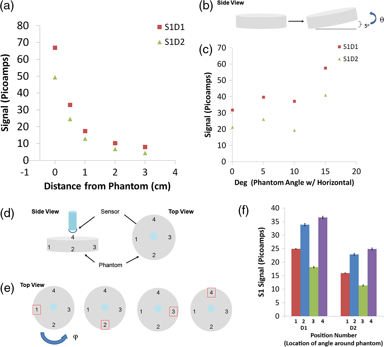$\text{mean of signal}\pm \mathrm{standard}\mathrm{deviation}$.

Table 4

Precision of signal as measured by coefficient of variation for the S1 sensor due to change in distance between phantom and sensor.

Table 5

Precision of signal as measured by coefficient variation for the S1 sensor during change in angle between phantom and sensor.

Table 6

Precision of signal as measured by coefficient variation for the S1 sensor during rotation of 5-deg angle of phantom to horizontal at four different positions.

3.4.

Determination of Variation in Sensor Signal for In Vitro, Fluorescent Phantom, and Live Mouse Fluorescent Sensing

We performed in vitro experiments to determine repeatability between the two sensors in the presence of fluorescence. We varied the concentration between 250, 500, 2500, and 10,000 nM. With the sensor fixed below a clear well containing Cy5.5 dilutions, the S1 sensor output signal varied linearly with fluorophore concentration, as did the S2 sensor [Fig. 4(a), $N=5$ measurements per concentration]. We compared the linearity and variation at each point with the S2 sensor and observed similar results [Fig. 4(b)]. To compare variations between detectors for each sensor, we plotted the mean value of one detector versus the mean value of the other detector at each concentration [Fig. 4(c)]. The data demonstrates that between each sensor, the signals correlate linearly [Fig. 4(c), arrows], but not in a one-to-one fashion. This can be appreciated by comparing the line for S1 (blue) or S2 (red) to the line for “$y=x$.” Because of the linear relationship between detector signal and concentration, it is possible to calibrate the two sensors, but for characterization studies we use only raw data from each sensor. Repeatability, as measured by a variation in signal after repeat measurements, ranged from $<0.92\%$ (250 nM), $<0.69\%$ (500 nM), $<6.77\%$ (2500 nM), and $<3.25\%$ (10,000 nM), and similar results were obtained with the D2 detector and with the S2 sensor.

Fig. 4

Determination of effects of in vitro, phantom, and live mouse fluorescent sensing on sensor signal. (a) Plot of signal versus concentration of fluorophore for S1 sensors in vitro. Comparison is made between two detectors (D1 and D2) for the S1 sensor. 100 µl of Cy5.5 fluorophore is placed in one microwell of a standard 96 microwell plate, and sensor is placed vertically above the well at a distance of 2 mm. Ten measurements were made and averaged; this was repeated several times for each concentration and presented as $\text{mean of signal}\pm \mathrm{standard}\mathrm{deviation}$ ($N=6$). Four concentrations were tested here and data from both S1D1 and S1D2 is shown; (b) same data as in (a), except a plot of signal versus concentration of fluorophore for S1D1 and S2D1 detectors at each concentration; (c) same data as in (a), except a plot of the mean of the signal from detector 1 versus the mean of signal from detector 2 for S1 and S2 sensors, at each concentration. Two arrows point toward 2.5 mM (left) and 5.0 mm (right) for both the S1 sensor and S2 sensors. A plot of “$y=x$” (dashed) is shown as a reference; (d) experimental system for fluorescence phantom sensing consisting of submerged functional sensor in a container containing 0.6% intralipid solution at room temperature. A fixed, sealed, capillary tube phantom containing 50-µM dye at base of container was used to mimic dye emitting object. Container was placed on a translational stage that could be moved controllably in the $x$, $y$, and $z$ directions; (e) effects of distance from fluorescent phantom, on signal. Three experiments with a total of six detectors (two detectors per sensor) were performed. Mean and standard deviation was calculated at each depth. Signal was baseline corrected and normalized to maximum signal and averaged across all detectors; (f) effects of changes in lateral position of fluorescent phantom on signal. While keeping the depth constant, normalized signal was calculated at varying lateral distances from the capillary tube. Then depth is incremented and measurement is repeated. At zero capillary depth, the signal drops to 50% of normal at 0.75 mm lateral from the capillary, whereas at the 1.2 mm depth, the signal drop to 50% of the normal position at approximately 1.4 mm; and (g) plot of signal versus time for S1 and S2 sensor. Cy5.5 fluorophore at a concentration of 500 nm is injected subcutaneously on the right hindlimb of the mouse and detected by the S2 sensor. The S1 sensor is placed above the left hindlimb and no signal is detected.

We then wanted to determine repeatability in sensing of fluorescence in a phantom model. A glass capillary tube filled with 50 μM Cy5.5 was fixed inside a container of liquid phantom formulated with 0.6% intralipid in distilled water to model tissue scattering (${\mu }_s\text{'}=6{\mathrm{cm}}^{-1}$ at 700 nm). The sensor was fixed and submerged in the container. The container, containing the capillary tube and liquid phantom material, was translated on a stage relative to the sensor. To avoid any effects of submersion, we engineered two similar sensors to S1 and S2, just for fluorescent phantom experiments. We used a liquid fluorescence-emitting phantom filled with the Cy5.5 fluorophore (50 µM) [Fig. 4(d)]. We measured the signal while keeping the sensor fixed and moving the container in the $x$ or $y$ (laterally) or $z$ (axially) direction in relation to the sensor. As expected, variation in depth of fluorophore resulted in an exponential reduction in signal [Fig. 4(e)]. We first measured the repeatability with the fluorescence phantom, and the repeatability varied from less than 12.99% (CV% $N=2$ trials, $N=4$ detectors). We then normalized the data for each sensor, and, using this approach, the variation increases to 9.60% at the highest depth of 3.2 mm (CV%).

To further determine the source of potential error in movement and positioning, we determined the field of view of the sensor using the fluorescent phantom. We performed a two-dimensional (2-D) plot to determine lateral and depth resolution. Our data demonstrates the effect of lateral distance and height on signal [Fig. 4(f), $N=2$ trials, $N=4$ detectors]. At the center of the phantom ($y=0$), the sensed signal from a volume of tissue containing fluorophore is a weighted average, with 90% of the signal coming from the first 1.9 mm [Fig. 4(f)]. As expected, at greater depths, there is decreased lateral resolution, as expected due to multiple scattering events. Overall, our data can be used to estimate a field of view of approximately $2.5\times 2.5\times 2\mathrm{mm}$ ($\mathrm{L}\times \mathrm{W}\times \mathrm{H}$) for our studies.

To understand variation when detecting fluorescence in live mice, we injected different concentrations of fluorophore subcutaneously (directly underneath skin) and performed sensing, again with the S1 and S2 sensors used previously. A representative plot demonstrates the signal was stable for 600 s at a concentration of 500 nM [Fig. 4(g)]. We measured signal variation by calculating the CV% based on the variation with time. The signal typically varied within 5% of the mean, and both detectors behaved similarly.

3.5.

Continuous Dynamic Sensing of the Intravenously Injected Fluorophore

A molecular probe is commonly administered intravenously, typically via the tail vein in a mouse, which results in the probe being subject to biodistribution via blood vessels and elimination via kidneys and or the liver, resulting in a tissue time-activity curve for a given tissue region of interest. Since we wanted to perform sensing of dynamics of molecular probe in the presence of tumors, we first wanted to establish dynamic of sensing a fluorophore (without a targeting moiety) in the absence of tumor. To establish dynamic sensing we first measured the background signal for $\sim 1000\mathrm{s}$, then injected 5 nmol of Cy5.5 intravenously in a live mouse and acquired data for at least 4000 additional seconds. Two sensors were used, placed bilaterally near the hindlimb. A typical time-activity curve consisted first of a constant, stable background signal, then a brief increase, and finally a slow decrease [Fig. 5(a)]. During all stages, the two detectors of each sensor exhibited identical dynamic changes. We performed baseline correction of each to further understand differences in kinetics between the two sensors. Interestingly, after baseline correction, we found that the signal peak reaches approximately the same level, but the S2 signal clearly decays at a higher rate [Fig. 5(b)]. For example, after 4000 s, the S1D1 signal is approximately 36 pA and the S2D1 signal is approximately 23 pA. Assuming that differences in scattering are accounted for by background subtraction, our data suggests that the fields of view illuminated by S1 and S2 sensors are heterogeneous with respect to fluorophore kinetics. We then plotted the raw kinetic data on a detector 1 versus detector 2 plot, and labeled the portions that correspond to dynamic portions of the curve in Fig. 5(a) in Fig. 5(c). The data was co-linear for both sensors over the entire time-activity curve. To demonstrate the co-linearity of the lines quantitatively, we performed linear curve fitting for each line [Fig. 5(c)]. The slope of the curve for the S2 curve was 0.989, while for the S1 curve was 0.979 [Fig. 5(c)], suggesting co-linearity. Our data validates that signal variation was likely due to change in fluorophore concentration and not due to change in the individual detector itself, which would result in a change in co-linearity on a detector 1 versus detector 2 plot.

Fig. 5

Effects of intravenously injected fluorophore on sensor signal. (a) Plot of the signal from each sensor/detector combination versus time for a mouse injected with 5 nmol of Cy5.5 fluorophore intravenously via tail vein. Continuous data (every 20 s) acquired for approximately 1400 s prior to injection, and for a total of 4000 s, in an anesthetized nude mouse; (b) same data as in (a) except each curve has been baseline subtracted; (c) same data as in (a) except plot of the signal from detector D1 versus the signal of detector D2 for sensor S1 and for sensor S2. The labels correspond to those used in (a); (d) a plot of the signal for the S1 sensor for a mouse injected with 3 nmoles of Cy5.5 fluorophore intravenously, in which signal was perturbed by changing anesthesia during sensing, “A” at each point of perturbation. Five segments of each curve are labeled 1 to 5 and separated by points in which anesthesia, “A,” was changed; and (e) same data as in (d) except plot of the signal from detector D1 versus the signal of detector D2 for sensor S1 and for sensor S2; the labels correspond to those used in (d).

To further understand how physiological variation in the living subject (mouse) affects signal, we performed controlled perturbation during sensing. Our preliminary experiments demonstrated that signal was extremely sensitive to small but abrupt changes in inhaled anesthesia (isofluorane) concentration. Since hemoglobin absorbs light at the VCSEL biosensor’s excitation and emission wavelengths, we propose that the change in signal could be due to isofluorane’s known effects on vasomotor activity, blood flow, or neuromuscular-driven movement. After the mouse reached a steady state level of anesthesia based on breathing rate, we abruptly increased isofluorane concentration (by 25%) above the steady state level (typically 1% $\mathrm{v}/\mathrm{v}$). We performed this perturbation several times at equally spaced intervals (approximately 1000 s) [Fig. 5(d), labeled as “$A$” to represent changes in anesthesia]. Overall, there are five distinguishable segments of signal, which are numbered with arrows [Fig. 5(d)]. Each perturbation resulted in an abrupt change in signal that could be clearly observed. To understand whether the detectors behaved in a co-linear fashion, we plotted the data in each of these segments on a detector 1 versus detector 2 plot [Fig. 5(e)]. Even after perturbation, the data appears to be co-linear, as evidenced by the different color segments, which appear to follow the same slope, as shown with linear curve fits [Fig. 5(e)]. For example, the slope of segment 4 (red) was 0.714, while the slope of segment 3 was 0.774 (blue). This indicates that despite the change in signal for the sensor, the signal from both detectors changes coordinately. We conclude that our sensor captures the entire time-activity curve during continuous sensing. Additionally, our data suggests that changes in signal due to clearance of probe and dynamic changes during perturbation signal can be detected. In the presence of perturbation, the two detectors in each sensor continue to behave in a coordinate fashion. Last, we demonstrate that different sensors in different locations in the same mouse can demonstrate kinetic differences that signify heterogeneity between the two fields of view.

3.6.

Quantitation of Continuous Sensing of the RAD-Cy5.5 and RGD-Cy5.5 Molecular Probes

Having established both precision and repeatability in the absence and presence of fluorophore, our goal was to noninvasively and continuously sense molecular probe in tumors. We chose the cRGD-Cy5.5 optical imaging probe and U87 tumor model, which are well-established molecular imaging probe and tumor models. We first chemically synthesized cRGD-Cy5.5 (RGD) [Fig. 6(a)] and the control, nontargeting probe, cRAD-Cy5.5 (RAD) and ensured the compounds were pure. We established that these probes function as expected using a small animal fluorescence imager with a cooled CCD camera. We injected tumor-bearing mice with 3 nmol of RAD ($N=3$ mice) and RGD ($N=3$ mice) via tail vein and imaged continuously for 2 h. As expected, fluorescence emission was greater in tumors of animals injected with RGD compared to RAD [Fig. 6(b), black arrows]. The mean tumor to background ratio (ratio of average radiance) from the tumor compared to the contralateral hindlimb (background) was significantly higher for RGD compared to RAD injected mice [Fig. 6(c), $p<0.05$], validating the targeting of the RGD probe compared to the control RAD probe.

Fig. 6

Continuous sensing of the RAD-Cy5.5 and RGD-Cy5.5 molecular probes in tumor-bearing mice. (a) Chemical structure of c(RGDyK)-Cy5.5. The c(RADyK)-Cy5.5 has alanine(A) substituted instead of glycine(G); (b) representative image of nude mice bearing U87 tumor xenografts injected via tail vein with 3 nmol of cRGD-Cy5.5 ($N=3$, left) or 3 nmol cRAD-Cy5.5 ($N=3$, right) acquired using a cooled CCD camera. Mice were anesthetized, injected simultaneously, and sequentially imaged for 2 h. Emission was filtered using a Cy5.5 filter. Tumor is located on right hindlimb of each mouse (black arrow); (c) plot of signal-to-background ratio versus time for the same mice in (b) continuously imaged with cooled CCD camera. Quantification performed on images of cRGD-Cy5.5 injected ($N=3$) and cRAD-Cy5.5 injected ($N=3$) mice using average radiance ($\text{photons}/\sec /{\mathrm{cm}}^2/\mathrm{sr}$). Data presented as $\text{mean}\pm \text{deviation}$; (d) double plot of averaged RAD data for S1 and S2 sensors (left axis) and S2D1 to S1D1 ratio (right axis). Tumor-bearing mice ($N=3$) were injected with the cRAD-Cy5.5 (nontargeted) probe and dual sensing was performed for 2 h. For mouse 1, the tumor was sensed by the S1 sensor; for mouse 2 and 3, the tumor was sensed by the S2 sensor; (e) plot of the averaged S2D1 to S1D1 ratio ($\text{mean}\pm \text{deviation}$) for tumor-bearing mice injected with the cRAD-Cy5.5 (control nontargeted, $N=3$) probe and cRGD-Cy5.5 (targeted, $N=5$) probe. Dual sensing was performed for 2 h; and (f) same as in (e), but averaged, calibrated S2D1 to S1D1 ratio is also shown in green. Calibration was performed by dividing averaged cRGD-Cy5.5 data by the averaged cRAD-Cy5.5 data.

We then performed more experiments with the RAD and RGD probes in tumor-bearing mice using S1 and S2 sensors. To better understand the dual-sensing approach, we first analyzed the signal due to fluorescence by comparing the signal from S1D1 and S2D1 in a variety of fluorescence data sets. For all fluorescence data sets, we performed baseline correction. We determined that for in vitro dye studies at various concentrations (500 nM, 2.5 µM, 10 µM) the S2D1 to S1D1 ratio was $0.644\pm 0.02$. For all live mouse studies, the ratio was 0.652 and 0.589 at 2 h after injection of dye alone, in mouse #1 and mouse #2, respectively, for S2D1 to S1D1 ratio. When we injected tumor-bearing mice with the nontargeted RAD, which does not accumulate in tumors, we again calculated the S2D1 to S1D1 ratio. We plotted the averaged signal of S1D1 and S2D1, as well as the average ratio of these two [Fig. 6(d)]. The average S2D1 to S1D1 ratio after RAD injection was $0.542\pm 0.049$ at 30 min, $0.523\pm 0.069$ at 1 h, $0.476\pm 0.092$ at 1.5 h, and $0.49\pm 0.113$ at 2 h. In the RAD experiments, the tumor was on the S2 side in one of the mice and on the S1 side in two other mice. Nevertheless, the ratio across several experimental systems was quite similar, and in all cases S2D1 was less than S1D1, and the ratio ranged from 0.476 to 0.542 for all RAD studies.

Next we evaluated the ratio of S2 (tumor side) to S1 (control side), after baseline correction, for tumor-bearing mice injected with RGD. The average S2D1 to S1D1 ratio after RGD injection was $1.236\pm 0.539$ at 30 min, $1.254\pm 0.524$ at 1 h, $1.362\pm 0.603$ at 1.5 h, and $1.662\pm 0.75$ at 2 h. We plotted the ratio for RAD and RGD injected mice together [Fig. 6(e), $\mathrm{mean}\pm \mathrm{S}\mathrm{.}\mathrm{D}$, $p<0.05$]. We observed statistically significant differences at all time points, and the curves appeared nearly identical to the case of analysis using the cooled CCD camera. Finally, we wanted to perform a calibration. Our simplest approach was to scale the RGD data by dividing each point by the RAD curve. This assumes that ratio of the two sensors for RAD injected mice should be 1, as we observed with images of our cooled CCD camera data. To normalize the RGD data to the RAD data, we performed a point-by-point division such that each point in the RGD ratio is divided by each point in the RAD ratio at each time. This resulted in a tumor-to-background similar to the cooled CCD camera data as shown [Fig. 6(f)]. For the calibrated ratio, the average S2D1 to S1D1 ratio was $2.367\pm 1.029$ at 0.5 h, $2.437\pm 0.950$ at 1 h, $2.929\pm 1.274$ at 1.5 h, and $3.640\pm \mathrm{0.1.379}$ at 2 h. This compares favorably with in vivo studies performed previously.³⁴

3.7.

Kinetics of Molecular Probe in Individual Mice During Continuous Sensing of the RAD-Cy5.5 and RGD-Cy5.5 Molecular Probes

Since many biological processes are dynamic with varying time and length scales, the ability to assess signal kinetics, and perform continuous imaging in each field of view has important implications for assessing functional differences of molecular probes. By using a dual-sensing strategy, we obtained quantitative information of the fluorescent molecular probe. Normally, after probe injection, dynamic signal from a single sensor was similar [Fig. 7(a)], with different magnitudes. We normalized the signal and compared signal after RAD injection from the same S1D1 detector across different mice. A wide range of signal dynamics was present between the same RAD probe across different mice [Fig. 7(b), $N=3$]. Furthermore, we compared the kinetics of RGD probe in mice bearing U87 tumors. Interestingly, we again observed a wide range of decay kinetics over 2 h, ranging from approximately 90% to 30% of initial signal, 2 h after injection [Fig. 7(c), $N=5$, $N=3$ shown]. Last, we compared the signal kinetics between tumor and normal tissue in an individual mouse, after injection of RGD. In both cases, the signal to background ratio was greater than 2, when we examined the absolute signal. Surprisingly, we found two different kinetic patterns. In one case, the RGD signal was decreasing faster in the normal tissue than the tumor [Fig. 7(d)], reaching approximately 60% and 30% of initial signal, respectively. In another case, the RGD signal decreased at the same rate in normal and tumor tissue and was approximately 85% after 2 h [Fig. 7(e)]. Our data demonstrates that the VCSEL-biosensor can also be used to study normalized data. Thus, the relative difference in kinetics of molecular probes in mice can be quantitatively measured. Using this approach, we measured differences between mice, between probes, and between tissue types (tumor versus normal).

Fig. 7

Kinetics of molecular probe in individual mice during continuous sensing of the RAD-Cy5.5 and RGD-Cy5.5 molecular probes. (a) Representative, baseline-corrected raw data plot of sensor signal versus time for S1D1 and S2D2 in nude mice bearing U87 tumor xenografts injected via tail vein with 3 nmol of cRAD-Cy5.5; (b) baseline-corrected, normalized data plot of sensor signal versus time for S1D1 for thee individual nude mice bearing U87 tumor xenografts injected via tail vein with 3 nmol of cRAD-Cy5.5; (c) baseline-corrected, normalized data plot of sensor signal versus time for S2D1 in individual nude mice bearing U87 tumor xenografts injected via tail vein with 3 nmol of cRGD-Cy5.5. S2 was sensing tumor in mouse 1, and S1 was sensing tumor in mouse 2 and 3; (d) baseline-corrected, normalized data plot of sensor signal versus time for S1D1 and S2D1 for individual nude mice bearing U87 tumor xenografts injected via tail vein with 3 nmol of cRGD-Cy5.5. Same as mouse #1 from (c); and (e) baseline-corrected, normalized data plot of sensor signal versus time for S1D1 and S2D1 for individual nude mice bearing U87 tumor xenografts injected via tail-vein with 3 nmol of cRGD-Cy5.5. Same as mouse #3 from (c).