2.1.

Coherent Backscattering

Detailed discussion of the nature of the CBS phenomenon can be found in a number of different publications.^3–7,17 Briefly, the experimentally measurable CBS peak shape $I_{\mathrm{CBS}}({\theta }_x,{\theta }_y)$ is the Fourier transform of the product of four functions:

Within the Fourier integral of Eq. (1), functions $p(x_s,y_s)$ and $pc(x_s,y_s)$ represent sample dependent properties that we will simulate numerically using electric field Monte Carlo while functions $s(x_s,y_s)$ and $c(x_s,y_s)$ are instrumental properties that can be found analytically as follows: Function $s(x_s,y_s)$ can be calculated as the normalized autocorrelation of the spatial illumination intensity distribution $A(x,y)$ incident on the scattering sample:^3,17

2.2.

Numerical Calculation of Functions $p(x_s,y_s)$ and $pc(x_s,y_s)$ with Monte Carlo

Electric field Monte Carlo simulations provide a numerical solution to the vector radiative transport equation in situations where an analytical solution is either difficult or impossible to derive. The basic structure of a light Monte Carlo code is well known. In brief, photons are first injected into a material and allowed to propagate according the material properties until the photon is either absorbed or exits the medium. Along the way, the polarization state of each photon is tracked and any number of parameters characterizing light propagation (e.g., reflectance, absorbance, time of flight, etc.) can be calculated.

For simulation of CBS, the interference between time-reversed photon path-pairs must be considered. One way to rigorously treat this coherence property is using the Jones calculus formalism to track the evolution of the electric field as it encounters optical components (e.g., polarizers), refractive index contrasts that induce scattering, and birefringent materials.³¹ In our simulations, which use a heavily modified version of the Stokes vector meridian plane Monte Carlo code written by Ramella-Roman et al.,³² the electric field undergoes four linear transformations for each scattering event:

For a multiple scattering sample, the transformations in Eq. (5) accumulate for each scattering event until the light escapes from the medium:

Generalizing the matrix $\overline{\mathbf{M}}$ for the forward propagating path (denoted with subscript $\odot$) we can write:

In order to maintain conservation of energy, we score all photons that exit outside of our grid or are single scattered in the peripheral pixels of each grid. In this paper, we normalize function $p(x_s,y_s)$ such that the integral over all spatial coordinates plus the single scattered intensity for unpolarized light equals 1:

Since CBS is a coherence phenomenon, it is required that both the polarization and phase of the time-reversed photon path-pairs are the same in order for interference to occur. As a result, function $p(x_s,y_s)$ is never independently measurable using CBS and instead can only be measured as the product of $p(x_s,y_s)·pc(x_s,y_s)$. One caveat of this statement is that for the polarization preserving channels (e.g., $xx$ and $++$), the reciprocity theorem requires that the forward and reverse propagating paths exit with the same accumulated phase and $pc(x_s,y_s)=1$. For the polarization nonpreserving channels (e.g., $xy$ and $+-$) the degree of coherence DOC for a single time-reversed path-pair is found as:⁸

2.3.

Computation of the Amplitude Scattering Matrix $\mathbf{S}(\theta ,\varphi )$ and Phase Function $\mathbf{P}(\theta ,\varphi )$

The amplitude scattering matrix $\mathbf{S}(\theta ,\varphi )$ in Eq. (5) succinctly summarizes the effects that a single scattering event has on the transformation of the incident electric field. For an arbitrary scattering media, each of the four matrix elements is independent of the others and are a function of both the polar angle $\theta$ and the azimuthal angle $\varphi$. However, a number of simplifications to the elements of $\mathbf{S}(\theta )$ can be made through knowledge about the geometry and composition of the scattering material. In media composed of spherically symmetrical scatterers (e.g., spheres or statistically homogeneous random media), the matrix elements $S_3$ and $S_4$ are identically equal to zero and the matrix elements $S_1$ and $S_2$ are solely functions³³ of $\theta$. In this paper, we implement two spherically symmetrical models for the composition of the scattering material: first, discrete spheres and second, statistically homogeneous continuous random media with refractive index distributions specified by the Whittle-Matérn family of correlation functions.^{1,17,24,36,37}

2.3.2.

Continuous random media—Born approximation

The Born approximation, also known as Rayleigh-Gans-Debye theory, provides a simplification to scattering theory which enables solutions for otherwise intractable problems (e.g., scattering in continuous random media). Provided that the fluctuations in refractive index are sufficiently weak such that the phase shift of the incident wave is small, we can approximate the total field within the scattering medium as the incident field. The scattered field can then be computed as the coherent summation of the dipole scattering pattern from each position within the medium. In the following paragraphs, we begin by describing the calculation of the scattering amplitude matrix under the Born approximation. We then apply these calculations to computation of scattering for a continuous random media defined under the Whittle-Matérn model.

The scattering amplitude matrix for an infinitesimal dipole can be found as:^33,35

Eq. (17)

$$\mathrm{d}\mathbf{S}(\theta )=-i{k}^3·\mathrm{d}\alpha ·\left[\begin{array}{cc}\cos \theta & 0\\ 0& 1\end{array}\right],$$

where $\mathrm{d}\alpha$ is the differential polarizability and $k$ is the wavenumber. For weak refractive index contrast $\mathrm{d}\alpha$, can be approximated as:

Eq. (18)

$$\mathrm{d}\alpha \approx \frac{n_{\mathrm{\Delta }}}{2\pi }\mathrm{d}V,$$

where $n_{\mathrm{\Delta }}$ is the excess refractive index within the differential volume $\mathrm{d}V$ relative to the mean medium refractive index $[(n_{\mathrm{d}V}/\langle n_{\text{medium}}\rangle )-1]$. To find the total scattered field for the ensemble scattering medium, we coherently sum the contribution from each dipole over the entire volume:

Eq. (19)

$$\mathbf{S}(\theta )=-i{k}^3·{\int }_V\frac{n_{\mathrm{\Delta }}(\overrightarrow{r})}{2\pi }{e}^{i{\overrightarrow{k}}_s·\overrightarrow{r}}\mathrm{d}V·\left[\begin{array}{cc}\cos \theta & 0\\ 0& 1\end{array}\right],$$

where $|{\overrightarrow{k}}_s|\equiv 2|\overrightarrow{k}|\sin \frac{\theta }{2}$. The term $e^{i{\overrightarrow{k}}_s·\overrightarrow{r}}$ accounts for the relative phase difference of the field originating from different positions within the medium and observed in the direction ${\overrightarrow{k}}_s$. Upon inspection, we see that the integral in Eq. (19) is essentially the three dimensional Fourier transform of $n_{\mathrm{\Delta }}(\overrightarrow{r})$.

For continuous random media, there is no elementary scattering particle with decipherable boundaries. As such, scattering must be defined in terms of the amplitude scattering matrix per unit volume polarizability $\mathbf{s}(\theta )$:

Eq. (20)

$$\mathbf{s}(\theta )=-i{k}^3·f(k_s)·\left[\begin{array}{cc}\cos \theta & 0\\ 0& 1\end{array}\right],$$

where function $f$ is the scattering form factor of the particular scatterer under investigation. Assuming spherical symmetry for the scattering medium, function $f$ can be calculated through reduction of the three dimensional Fourier transform in Eq. (19):

Eq. (21)

$$f(k_s)=\frac{2}{\alpha }{\int }_0^{\infty }{M}_n(r)\frac{r\sin (k_{s}r)}{k_s}\mathrm{d}r,$$

Eq. (22)

$$\alpha =2{\int }_0^{\infty }{r}^2{M}_n(r)\mathrm{d}r,$$

where the statistical function $M_n(r)$ is the particulate equivalent medium and replaces $n_{\mathrm{\Delta }}(\overrightarrow{r})$ in Eq. 19. Conceptually, $M_n(r)$ can be thought of as the effective particle which gives the same scattered intensity as the random process described by $n_{\mathrm{\Delta }}(\overrightarrow{r})$ [see Fig. 1(a)]. Note that $M_n(r)$ uses the scalar $r$ (implying spherical symmetry), while $n_{\mathrm{\Delta }}(\overrightarrow{r})$ uses the vectorial $\overrightarrow{r}$ (implying lack of symmetry).

Fig. 1

Numerical validation of our treatment of scattering using function ${\mathit{M}}_n(r)$. (a) Randomly generated 3-D medium under the Whittle-Matérn model for $D=3$. (b) Comparison of function $|f|$ calculated numerically and analytically for the medium shown in panel a.

One attractive model for $M_n(r)$ in a continuous random scattering medium originates from the Whittle-Matérn family of correlation functions.³⁷ Under this model, the distribution of refractive index fluctuations is defined through the medium’s refractive index correlation function $B_n(r_s)$:

Eq. (23)

$$B_n(r_s)=A_n{\left(\frac{r_s}{l_c}\right)}^{\frac{D-3}{2}}{K}_{\frac{D-3}{2}}\left(\frac{r_s}{l_c}\right),$$

where $K_{\nu }$ is the modified Bessel function of the second kind with order $\nu$, $l_c$ describes the length-scale of tissue heterogeneity, $A_n$ is the fluctuation strength, and $D$ is a parameter which determines the shape of the distribution (e.g., Gaussian, stretched exponential, exponential, and power law distributions).³⁷ Implementation of the Whittle-Matérn model provides the flexibility to mimic the distributions of refractive index expected for a wide range of different biological tissue types.^18,24,37 It should be noted that when $D=3$, this model predicts a scattering phase function that is identical to the commonly used Henyey-Greenstein case. Figure 1(a) shows a single realization of the three dimensional excess refractive index distribution for $D=3$.

According to the convolution theorem, the random process $n_{\mathrm{\Delta }}(\overrightarrow{r})$ is related to $B_n(r_s)$ and $M_n(r)$ by:

Eq. (24)

$$\begin{gathered} B_n(r_s)={\mathcal{F}}^{-1}[{|\mathcal{F}[n_{\mathrm{\Delta }}(\overrightarrow{r})]|}^2] \\ ={\mathcal{F}}^{-1}[{|\mathcal{F}[M_n(r)]|}^2], \end{gathered}$$

where the symbol $\mathcal{F}$ indicates the Fourier transform operation. Inverting Eq. (24), we can derive $M_n(r)$:

Eq. (25)

$$M_n(r)=\frac{2\sqrt[4]{2}{\pi }^{3/4}\sqrt{A_n\mathrm{\Gamma }(D/2)}}{\mathrm{\Gamma }(D/4)l_c^{3/2}}{\left(\frac{r}{l_c}\right)}^{\frac{D-6}{4}}{K}_{\frac{D-6}{4}}\left(\frac{r}{l_c}\right).$$

It should be noted that $M_n(r)$ is a statistical function that provides the same information as $B_n(r_s)$ but allows for the calculation of the scattered electric field needed for electric field Monte Carlo. One caveat of the previous statement is that the phase information is not represented and so we can only correctly calculate the modulus of function $f$. Still, the shape of the scattering phase function which is proportional to the square of function $\left|f\right|$ is unaffected by this distinction. Performing the integrations in Eqs. (21) and (22), under the Whittle-Matérn model function $\left|f\right|$ can be found as:

Eq. (26)

$$|f(k_s)|={(1+k_s^2{l}_c^2)}^{-D/4}.$$

Equation (26) is an accurate estimate of scattering provided ${\sigma }_n^2{(k{l}_c)}^2\ll 1$.³⁹

Figure 1 provides a numerical validation of our treatment of scattering using function $M_n(r)$. Figure 1(a) shows a three dimensional random medium generated using a publicly available code for $D=30$.⁴⁰ Using this medium, we calculated function $\left|f\right|$ by numerically computing the modulus of the three-dimensional (3-D) Fourier transform in Eq. (19), rotationally averaging the resulting function, and finally normalizing by the first point. Figure 1(b) shows a close match between this numerically calculated function and the analytical result from Eq. (26).

2.4.

Computation of the Jones $\mathit{M}$-Matrix for Implementation of Birefringence

A number of biological tissues exhibit some combination of linear birefringence due to structural alignment and optical activity due to the presence of chiral molecules. Since the matrix transformations of the electric field are noncommutative, the order in which these effects are applied can potentially alter the observable signal.⁴¹ In this paper, we assume a stochastic medium in which there is no preferential order for the effects of linear birefringence and optical activity. In order to combine these two effects into a single matrix operation, the Jones $\mathbf{N}$-matrix formalism can be utilized.³⁴

The Jones $\mathbf{N}$-matrix represents the transformation of the electric field for an infinitesimally small propagation path length $\mathrm{d}s$. Following the derivation by Jones, this enables the combination of multiple polarization-altering effects (e.g., birefringence and dichroism) into a single $\mathbf{M}$-matrix which represents a transformation over the entire path length. The $\mathbf{N}$-matrix for a specimen containing both linear birefringence and optical activity can be written as⁴¹:

The parameter $g_0$ can be found as:³⁴

The parameter $\omega$ can be found as the product of the chiral molecule’s specific rotation ${[\alpha ]}_{\lambda }^T$ at temperature $T$ (degrees Celsius) and its concentration $\rho$:

The $\mathbf{M}$-matrix elements corresponding to the convention in Eq. (4) can be calculated for a given path length $s$ as:

3.1.

Semi-Analytical Approach

In order to accurately model CBS, function $p(x_s,y_s)$ must be calculated for reflected light that is antiparallel to the incident direction. However, under the traditional Monte Carlo approach, only an infinitesimally small number of photons will exit the scattering medium exactly in this direction. As a result, in order to achieve any computational efficiency, it is necessary to collect all photons that exit the medium within some finite collection angle around the backscattering direction. Unfortunately, this generates a trade-off between computational accuracy and efficiency since the spatial distribution of light reflected at different angles is not constant. As a compromise, previous publications have found that collection of photons exiting the medium within an angle of 10 degrees around the backscattering direction produce no noticeable deviations from the theoretical shape of function $p(x_s,y_s)$.^18,23 Still, under the traditional approach only a relatively small number of the total photons contribute to the final result.

In order to improve the computational efficiency of the traditional approach to Monte Carlo simulations, we implement the semi-analytical approach (also known as the partial photon technique).^{8,27,28,42,43} Using this method, a portion of scattered intensity is collected after a photon reaches each new position within the medium. This “partial photon” intensity $I_{\text{partial}}$ is calculated by multiplying the probability that the photon is scattered in the direction of the surface $F({\theta }_s,0)$ by the probability that it will reach surface according to the Beer-Lambert law $e^{-({\mu }_s+{\mu }_a)z}$:

Figure 2 shows a visual comparison of the noise level between the semi-analytical (panel a) and traditional (panel b) technique in a Rayleigh scattering sample simulated for the $xx$ polarization channel. Figure 2(c) compares the $p_{xx}(r_s·{\mu }_s^{*})$ and $p_{xx}(z·{\mu }_s^{*})$ distributions achieved by summing $p_{xx}(r_s·{\mu }_s^{*},z·{\mu }_s^{*})$ over rows and columns, respectively. Note that since $p(r_s,z)$ scales linearly with the reduced scattering coefficient ${\mu }_s^{*}=1/l_s^{*}$, we show each distribution as a function of the dimensionless parameters $r_s·{\mu }_s^{*}$ and $z·{\mu }_s^{*}$. Quantitative comparison of the computational efficiency between the two techniques is shown in Fig. 2(d) and calculated by taking the ratio of the number of traditional photons over the number of semi-analytical photons needed to achieve the same simulation noise level. For isotropic scattering (i.e., $g=0$), the semi-analytical approach is an exceptional 200 times faster than the traditional approach. The efficiency of the semi-analytical approach decreases for increasing anisotropy factor, but remains superior for values of $g<0.96$ (which encompasses the majority of tissue types⁴⁴). In order to ensure optimal efficiency for each simulation, our code scores photons using both the traditional and semi-analytical technique.

Fig. 2

Comparison between the semi-analytical and traditional Monte Carlo method in a sample of Rayleigh scatterers simulated for the $xx$ polarization channel. Function $p_{xx}(r_s·{\mu }_s^{*},z·{\mu }_s^{*})$ for (a) the semi-analytical method and (b) the traditional method. (c) Functions $p_{xx}(r_s·{\mu }_s^{*})$ and $p_{xx}(z_s·{\mu }_s^{*})$ achieved by summing $p_{xx}(r_s·{\mu }_s^{*},z·{\mu }_s^{*})$ over rows and columns, respectively. The symbols indicate the traditional technique while the solid line indicates the semi-analytical approach. (d) Computational efficiency measured by taking the ratio of the number of traditional photons over the number of semi-analytical photons needed to achieve the same simulation noise level. These simulations utilize the Whittle-Matérn model with 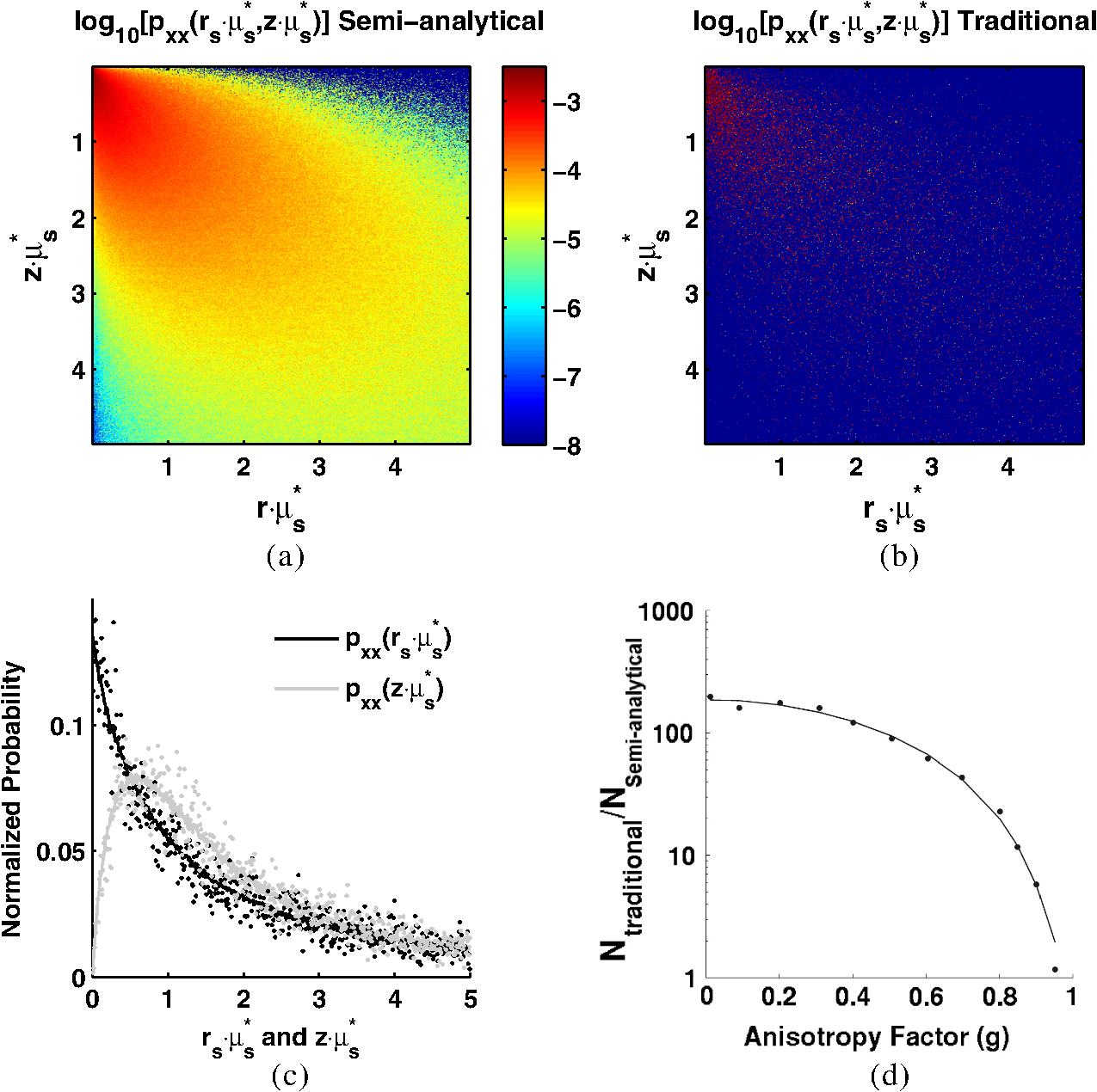$D=3$.

3.2.

MPI Implementation

One of the computational benefits of performing Monte Carlo simulations is that the noise level scales inversely with the number of recorded photons. Due to the stochastic nature of the Monte Carlo method, information from each photon is independent and calculations from an indeterminate number of processors can be linearly combined to reduce the noise variance. In order to take advantage of this capability, we have implemented MPI into our simulations. This allows multiple processors to independently calculate a predetermined number of photon histories, and subsequently combine the results after each processor has finished. A simulation of Rayleigh scattering for ${10}^8$ photons on a dual quadcore workstation (2.1 GHz AMD Opteron Processor 2352) can be run in less than 1.5 h.

3.3.

MATLAB GUI

Within the engineering community, MATLAB is the preferred platform on which to analyze data. However, to perform highly repetitive calculations in the minimum amount of time, the C programming language is advantageous. In order to combine the usability of MATLAB and speed of C code, we have implemented a software program that integrates these two environments. User interaction with the simulation is carried out through the MATLAB GUI shown in Fig. 3. After specifying the desired parameters, a simulation can be imported into a C code environment for rapid calculation of functions $p(x_s,y_s)$ and $pc(x_s,y_s)$ on multiple processors with a single button click. After the simulation is completed, all relevant data is automatically compiled and saved into a single MATLAB format file under a user specified file name.

Fig. 3

MATLAB GUI for performing Monte Carlo simulations of CBS. (a) Specification of the general Monte Carlo parameters. (b) Specification of scattering model to be implemented. (c) Specification of the birefringence properties of the sample.

The MATLAB GUI consists of three main panels used to specify the relevant simulation parameters. The panel in Fig. 3(a) allows the user to specify the general Monte Carlo parameters such as illumination polarization, photon and processor numbers, optical coefficients ${\mu }_s^{*}$ and ${\mu }_a$, as well as grid size and discretization. The panel in Fig. 3(b) enables simulations to be carried out using either a discrete sphere model under Mie Theory or a continuous distribution of refractive index under the Whittle-Matérn model as described in Sec. 2.3. The panel in Fig. 3(c) allows the user to set birefringence parameters such as the ordinary and extraordinary refractive index, the optical rotation, and the birefringence unit vector. Additionally, the GUI provides the capability to plot a summary of the simulation data as well as export data to and compile data from a remote computer cluster. Further specific details on the operation of the GUI can be found in a user manual posted along with our code.³⁰

4.1.

Trends for Purely Scattering Samples

For any particle form factor (spheres, continuous random media, etc.), the shape of the differential scattering cross-section converges to that of Rayleigh scattering when the characteristic length-scale of the particle is much smaller than the wavelength of illumination. Because of this common thread between all scattering form factors, we begin by analyzing the shape of the CBS peak for Rayleigh scattering.

One way to quantify the shape of the CBS peak is through the enhancement factor $E$ or the relative height of the peak at $\theta =0$ divided by the total unpolarized incoherent intensity. Mathematically, this can be found as:

Table 1 contains a summary of the values of $E$ in the various polarization channels for nonabsorbing Rayleigh scatterers with index matching at the boundary and results rounded to the fourth decimal place. Comparison with the benchmark values calculated by Mishchenko as well as Amic et al. using two separate numerical techniques show errors below 2% in each case.^45,46 Additionally, the value of $E_{xx}$ is in agreement with a Monte Carlo code which takes an alternative semi-analytic approach.⁴⁷ We note that the values given in Refs. 45 and 46 are converted into the normalization used in this paper before display in Table 1.

Table 1

Values of E in various polarization channels for nonabsorbing Rayleigh scatterers with index matching at the boundary. The values given for Refs. 45 and 46 are converted into the normalization used in this paper before display.

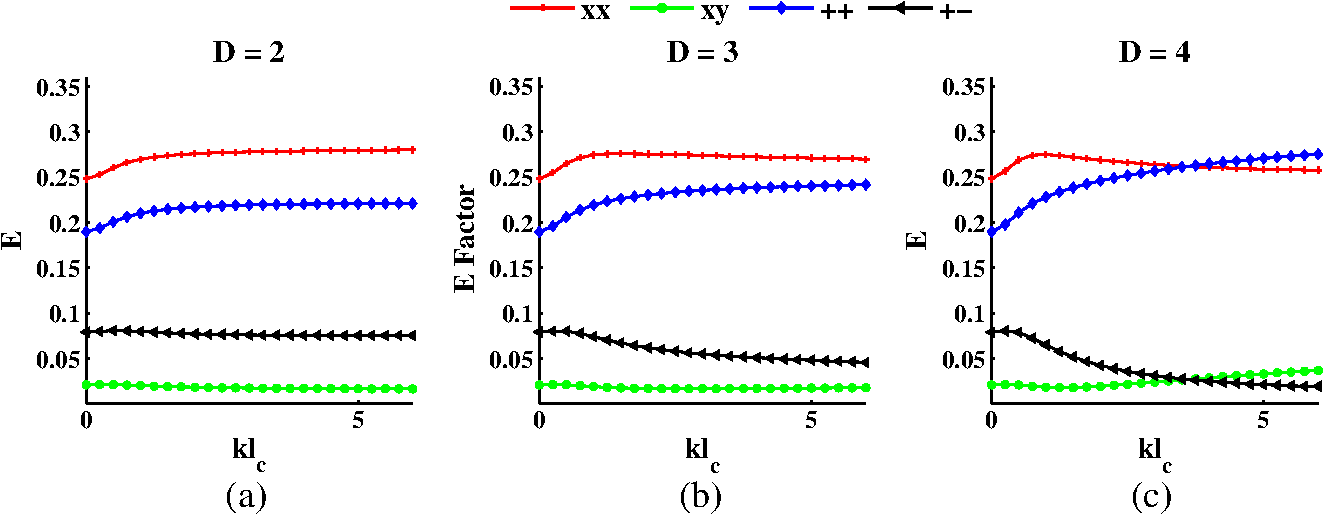
In the idealized scalar case $E$ would be exactly equal to 1, meaning that the coherent intensity is the same magnitude as the incoherent intensity. However, for real electromagnetic waves $E_{oo}$ is less than 1 due to first, single scattering and second, partially reversible photon paths (i.e., paths in which $\mathrm{DOC}\ne 1$). For the $xx$ and $++$ polarization preserving channels, function $pc(r_s)$ is identically equal to 1. Because of this, $E_{xx}$ and $E_{++}$ are nearly one quarter of the total unpolarized incoherent intensity. For the $xy$ and $+-$ orthogonal polarization channels, $E_{xx}$ and $E_{++}$ are greatly reduced due to the decay of function $pc$ at large values of $r_s$.

As the characteristic length-scale of the particle approaches the wavelength of illumination, the specific scattering form factor begins to dominate the shape of the differential scattering cross-section. Under Mie theory, the characteristic length-scale is the radius of the spherical particle, $a$. Figure 4 shows $E$ as a function of the dimensionless size parameter $ka$. Figure 4(a) shows these trends for a scattering medium with a relative refractive index $m=n_{\text{sphere}}/n_{\text{medium}}$ corresponding to polystyrene microspheres suspended in water. For very small $ka$, the results converge to the values of Rayleigh scattering given in Table 1. As $ka$ increases, the trends in each polarization channel exhibit an oscillatory pattern due to the spherical form factor. Interestingly, the trends shown in Fig. 4(a) remain essentially the same with the reduced refractive index contrast shown in Fig. 4(b) and 4(c). From these results it can be concluded that refraction of the light wave within the scattering particle has a smaller effect on the shape of the CBS peak than the underlying spherical particle scattering form factor.

Fig. 4

Enhancement factor $E$ versus size parameter $ka$ for various polarization channels under Mie theory. (a) Trends for relative refractive index $m=n_{\text{sphere}}/n_{\text{medium}}$ corresponding to aqueous suspension of polystyrene microspheres. (b) Trends for $m=1.1$. (c) Trends for $m=1.001$.

Under the Whittle-Matérn model, the characteristic length-scale is the parameter $l_c$. Figure 5 shows $E$ as a function of the dimensionless parameter $k{l}_c$ for various values of $D$. Similar to the Mie theory results above, for very small $k{l}_c$ the values converge to those of Rayleigh scattering. For larger values of $k{l}_c$, $E$ exhibits a smooth change trend due to the smoothly decaying form factor underlying scattering in the Whittle-Matérn model.

Fig. 5

Enhancement factor $E$ versus $k{l}_c$ for various polarization channels under the Whittle-Matérn model. (a) Trends for $D=2$. (b) Trends for $D=3$. (c) Trends for $D=4$.

4.2.

Effects of Birefringence

To demonstrate the general effects of biological birefringence on the shape of the CBS peak, we once again turn to the case of Rayleigh scattering. To study these effects within the biologically relevant regime,⁴⁸ we performed simulations for values of $\mathrm{\Delta }{n}_{b,\max }$ ranging from 0 to $1\times {10}^{-3}$ with a birefringence unit vector oriented along the $x$-axis (i.e., $\mathbf{b}=[1,0,0]$).

Figure 6 demonstrates the effects of linear birefringence on the spatial reflectance profiles for linear polarized illumination and collection with the arrows indicating increasing values of $\mathrm{\Delta }{n}_{b,\max }$. Noting that ${pc}_{xx}=1$ for all length-scales, Fig. 6(a) demonstrates that the $p_{xx}$ and $p_{xy}$ distributions which would be measured using conventional incoherent techniques exhibit minimal sensitivity to the presence of birefringence. However, a noteworthy change in the coherent $p_{xy}·{pc}_{xy}$ distribution (measurable using CBS) occurs even for small values of $\mathrm{\Delta }{n}_{b,max}$. The explanation for this observation is that the presence of birefringence reduces the reversibility of the path travelled by each multiply scattered photon, resulting in a more sharply decaying function ${pc}_{xy}$ shown in Fig. 6(b). Mathematically, the additional polarization rotations imparted by the presence of birefringence reduce the symmetry of the effective complex scattering matrix ${\overline{\mathbf{M}}}_{\odot }$ and therefore cause the forward and reverse propagating rays to be less correlated with each other on average.

Fig. 6

Effects of linear birefringence on the spatial reflectance profiles under linear polarized illumination and collection for a sample of Rayleigh scatterers. (a) The normalized intensity distributions $p_{xx}·{pc}_{xx}$ and $p_{xy}·{pc}_{xy}$ which are measurable using CBS. The dashed line indicates the shape of the incoherent $p_{xy}$ distribution which is not directly measurable using CBS. (b) Function ${pc}_{xy}$. Due to the full reversibility of the $xx$ polarization channel, ${pc}_{xx}=1$ for all length-scales. In both panels, the arrow indicates increasing $\mathrm{\Delta }{n}_{b,\max }=0$, $4\times {10}^{-4}$, $7\times {10}^{-4}$, and $1\times {10}^{-3}$.

Figure 7 shows the effects of birefringence on the spatial reflectance profiles for circularly polarized illumination and collection with increasing $\mathrm{\Delta }{n}_{b,\max }$. Similar to the effect described for linear polarization, function ${pc}_{+-}$ shown in Fig. 7(b) is more strongly decaying for large values of $\mathrm{\Delta }{n}_{b,\max }$. This results in a strong attenuation of function $p_{+-}·{pc}_{+-}$ relative to function $p_{+-}$ at large length-scales. Interestingly, for circular polarization both functions $p_{++}$ and $p_{+-}$ are altered at short length scales due to the presence of birefringence. The reason for this observation can be understood by considering the rotation of polarization that occurs due to birefringence prior to the first scattering event. As the circularly polarized photon enters the medium and propagates to the first scattering event, it encounters the birefringence material and becomes elliptically polarized. Thus, when the photon encounters the first scattering event, the shape of the scattering phase function is altered relative to the absence of birefringence case (note: although we use the first scattering event as conceptual description, the described effect will occur at each scattering event). The degree of alteration in the shape of the phase function is directly related to the strength of the birefringence; the stronger the birefringence, the larger the alteration in the phase function. Because of this change in the phase function, the shapes of $p_{++}$ and $p_{+-}$ are altered at short length scales due to the presence of birefringence. Further demonstration of this effect is seen in Fig. 8 with discussion found below.

Fig. 7

Effects of linear birefringence on the spatial reflectance profiles under circularly polarized illumination and collection for a sample of Rayleigh scatterers. (a) The normalized intensity distributions $p_{++}·{pc}_{++}$ and $p_{+-}·{pc}_{+-}$ which are measurable using CBS. The dashed line indicates the shape of the incoherent $p_{+-}$ distribution which is not directly measurable using CBS. (b) Function ${pc}_{+-}$. Due to the full reversibility of the $++$ polarization channel, ${pc}_{++}=1$ for all length-scales. In both panels, the arrow indicates increasing 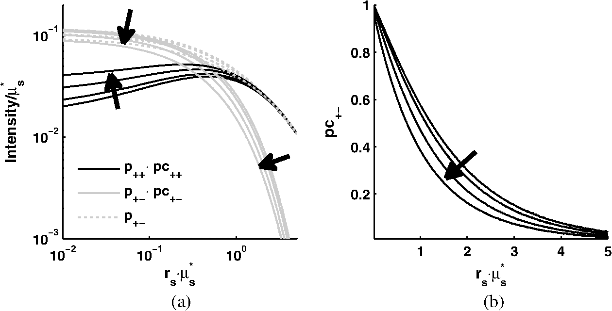$\mathrm{\Delta }{n}_{b,\max }=0$, $4\times {10}^{-4}$, $7\times {10}^{-4}$, and $1\times {10}^{-3}$.

Fig. 8

Alterations in the shape of $p(x_s,y_s)·pc(x_s,y_s)$ due to birefringence for different polarization channels. To emphasize the shape of the various distributions, each image shows ${\log }_{10}[p(x_s,y_s)·pc(x_s,y_s)]$ in the same intensity scale. (Rows) Each row corresponds to the polarization channel specified on the far right of the figure: top row shows $xx$ polarization, second row shows $++$ polarization, third row shows $xy$ polarization, and the bottom row shows $+-$ polarization. (Columns) The left column shows the ${\log }_{10}[p(x_s,y_s)·pc(x_s,y_s)]$ distributions for $\mathrm{\Delta }{n}_{b,\max }=0$ and the middle column shows the distributions for $\mathrm{\Delta }{n}_{b,\max }=1\times {10}^{-3}$. The right column shows the angular distribution found by converting to polar coordinates, summing over radius, and normalizing by the mean.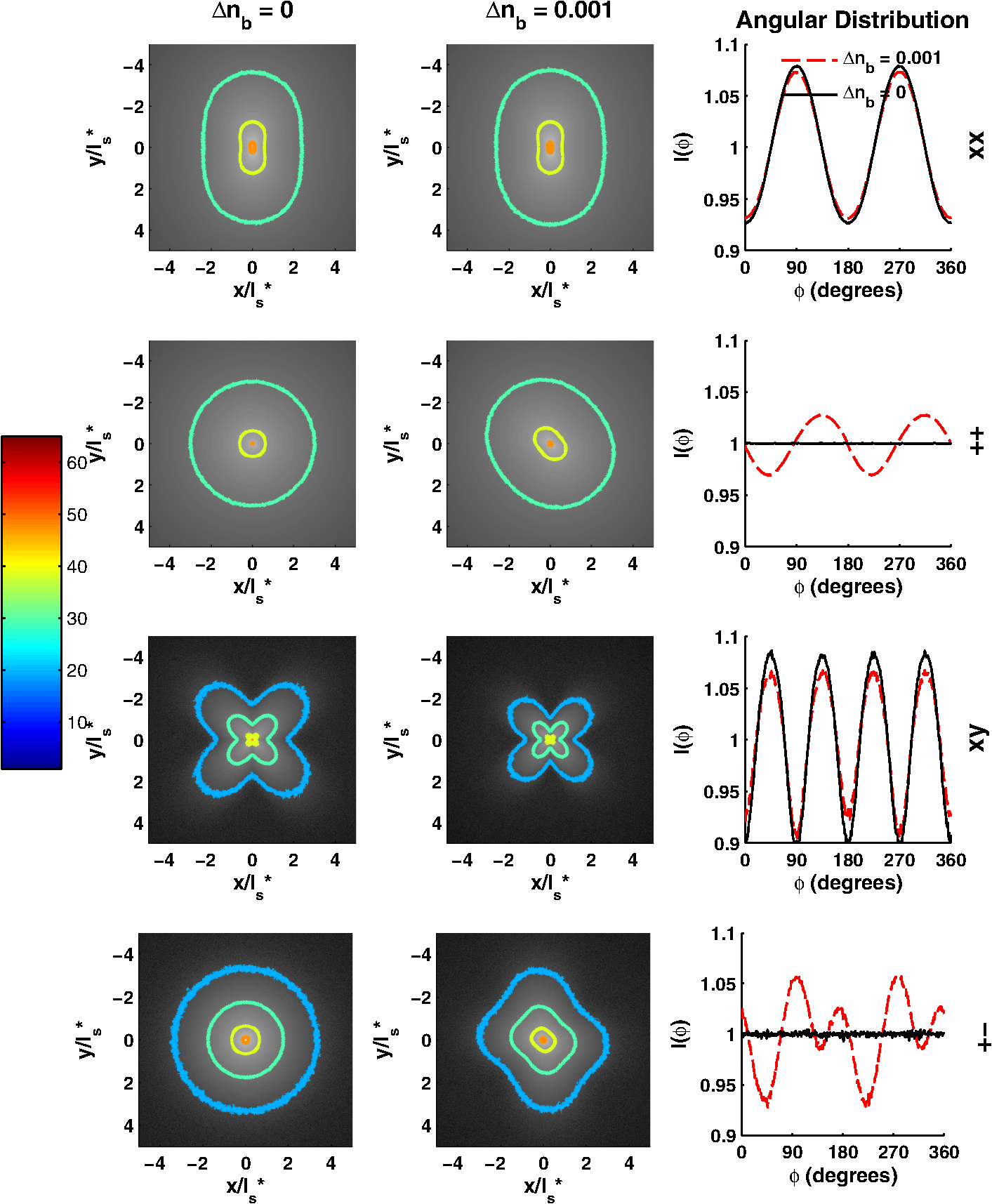

Trends of $E$ as a function of physiological levels of $\mathrm{\Delta }{n}_{b,\max }$ are shown in Fig. 9(a). Beginning with $\mathrm{\Delta }{n}_{b,\max }=0$, the values for $E$ are the same as in Table 1. As $\mathrm{\Delta }{n}_{b,\max }$ increases, the value of $E$ weakly increases for the polarization preserving channels and more strongly decreases for the orthogonal polarization channel. The percent change in $E$ for the various polarization channels relative to the absence of birefringence is shown in Fig. 9(b). For $\mathrm{\Delta }{n}_{b,\max }=1\times {10}^{-3}$ (on the order of the highest value found in biological tissue), there is an approximately 10% increase in $E$ for the polarization preserving channels attributable mainly to the change in the shape of the phase function. On the other hand, in the orthogonal polarization channels $E$ decreases by $\sim 37\%$ for the $+-$ channel and $\sim 50\%$ for the $xy$ channel due the destruction of reversibility attributable to the presence of birefringence.

Fig. 9

Changes in $E$ as a function of $\mathrm{\Delta }{n}_{b,\max }$ for various polarization channels. (a) Trends of versus $E$. (b) Percent change in $E$ from the absence of birefringence case versus 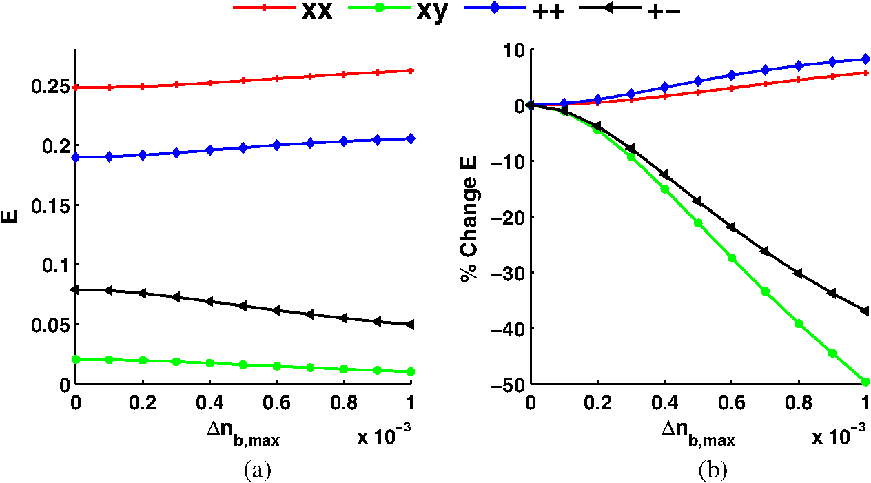$\mathrm{\Delta }{n}_{b,\max }$.

Figure 8 shows the comparison in the shape of $p(x_s,y_s)·pc(x_s,y_s)$ between $\mathrm{\Delta }{n}_{b,\max }=0$ (left column) and $\mathrm{\Delta }{n}_{b,max}=1\times {10}^{-3}$ (center column). The angular distribution shown in the right column is found by converting the Cartesian coordinates into polar coordinates, summing over radius, and normalizing by the mean. Each of the four rows corresponds to the polarization channel shown at the far right of the figure. Starting from the top row we show the $xx$, $++$, $xy$ and $+-$ polarization channels. In the top row, we observe a minimal change in the shape of $p_{xx}(x_s,y_s)$, while in the second row the shape of $p_{++}$ is noticeably elongated along the ${135}^{°}/{315}^{°}$ direction. The explanation for $++$ channel is that the incident right circular illumination becomes elliptically polarized along the $45\text{-}\mathrm{deg}/225\text{-}\mathrm{deg}$ direction as it propagates through the birefringent crystal. This causes a decreased probability of scattering in the direction of the ellipticity (known as the dipole factor)^17,37 which in turn results in more light intensity being scattered orthogonal to this direction. The direction of the elongation depends on the magnitude and sign of $\mathrm{\Delta }{n}_{b,\max }$ as well as the helicity of incident light. In the third row, the increased value of function $\mathrm{\Delta }{n}_{b,\max }$ shrinks the spatial extent of $p_{xy}(x_s,y_s)·{pc}_{xy}(x_s,y_s)$ due to a more strongly decaying function ${pc}_{xy}(x_s,y_s)$ as described above. Finally, in the last row the shape of $p_{+-}(x_s,y_s)·{pc}_{+-}(x_s,y_s)$ is altered from a symmetric shape to an oblong “X” shape with increasing birefringence. The reason for this shape is the conversion of the incident circular light to an elliptical state that mimics the “X” pattern of the $xy$ polarization channel.