

|
|
1.IntroductionOvarian cancer has the lowest survival rates of the gynecologic cancers because it is predominantly diagnosed in stages III and IV due to the lack of reliable symptoms as well as the lack of efficacious screening techniques.1 Currently, there is no single test for ovarian cancer, the combination of the serum marker CA125 screening (sensitivity of less than 50%),2–4 transvaginal ultrasound (3.1% positive predictive value),5 and pelvic exams (sensitivity of only 30%) yields low positive predictive value.2 Computed tomography (CT) scan has been studied extensively for ovarian cancer detection and multiple studies confirm that CT has a sensitivity of 45%, a specificity of 85%, a positive predictive value of 80%, and a negative predictive value of 50%.6 It is poor in detecting small metastases of less than 2 cm in diameter. MRI has not been shown to have a significant advantage, although it may be superior to CT for characterizing malignant features of an ovarian mass and is often used when ultrasound is not diagnostic.7 However, magnetic resonance imaging (MRI) is costly and typically used as a secondary imaging method. Positron emission tomography (PET), using 18F-FDG as a tracer, can detect malignant cancers with altered glucose metabolism and has been used for the assessment of lymph node involvement,8 evaluation of pretreatment staging and treatment response,8,9 and detection of cancer metastases. However, it has limited value in lesion localization in early stages of ovarian cancer because of the difficulty in distinguishing between the signal from early-stage cancers and the background uptake signals coming from the normal tissue.10 In recent studies, multi-parametric ultrasound and clinical analysis scoring systems showed a superior performance in diagnosing adnexal masses. The scoring systems are based on subjective scoring of some biographical, morphological, and clinical parameters, e.g., age of the patient, CA125 test, some sonographic features, such as size of the ovary, inner wall structure, thickness of the wall, presence of cysts, presence and type of septations and papillations, color in Doppler flow signals (vasculature of tumor), etc. After subjective scoring, various mathematical models were constructed to improve diagnosis, and the performances of the models were compared thoroughly. They reported that simple scoring systems performed the worst overall, whereas multitechnique risk of malignancy index models performed better and similar to that of most logistic regression and artificial neural network (NN) models. The most accurate results were obtained with a relevance vector machine (similar to SVM) model, with the use of these complex mathematic models resulting in the correct diagnosis of a significant number of additional malignancies.11–14 Photoacoustic tomography (PAT) is an emerging technique in which a short-pulsed laser beam penetrates diffusively into a tissue sample.15–18 The transient photoacoustic waves generated from thermoelastic expansion resulting from a transient temperature rise are then measured by ultrasound transducers, and used to reconstruct, at ultrasound resolution, the optical absorption distribution that reveals optical contrast, which is directly related to the microvessel density of tumors or tumor angiogenesis.19 Angiogenesis is a key process for tumor proliferation, growth, and metastasis.20 These functional parameters are critical in the initial diagnosis of a tumor and in the assessment of tumor response to treatment. The penetration depth of PAT is scalable with ultrasound frequency, provided that the signal-to-noise ratio (SNR) is adequate. In the diagnostic frequency range of 3 to 8 MHz, the penetration depth in tissue can reach up to 4–5 cm using near infrared (NIR) light,21 which is compatible with the penetration depth used in conventional transvaginal ultrasound. We have introduced coregistered photoacoustic and ultrasound imaging for detection and characterization of malignant and benign ovarian tissues.21–23 This new approach allows us to visualize tumor structure and functional changes simultaneously, which may potentially reveal early tumor angiogenesis development that is not available by ultrasound alone. Our recent study evaluated 33 ex vivo ovaries with diverse pathological conditions using a coregistered photoacoustic and ultrasound system and showed that malignant ovaries exhibited on average a much higher total absorption than normal ovaries. The quantitative parameter used to evaluate the absorption is the measured average maximum radio-frequency PAT signal for each ovary, with the maximum taken at each ultrasound array element and the average taken across all the array elements. Using this measure, we obtained sensitivity of 83% and a specificity of 83% between malignant ovaries and normal ones () in the postmenopausal group. This result suggests that photoacoustic imaging is a promising modality for improving ultrasound diagnosis of ovarian cancer. Automated identification of ovarian cancer from confocal microendoscopic images showed promising results that can be effective in assisting physicians with diagnosis and guiding biopsies.24 In this study, we introduce an automated algorithm for recognition of ovarian cancer from coregistered ultrasound and photoacoustic images. PAT provides high resolution images of vascular distribution features that can be used for assisting diagnosis of malignant and benign ovaries, whereas ultrasound images reveal many morphological features that can be used as classifying features that may be unique to some physiological processes of the complex ovaries and distinguishing them from malignant patterns. The need for utilizing more features for improving the diagnosis of malignant cancers from benign ovarian tissues and lack of literature data in this area has motivated our study reported in this paper. 2.MethodsIn this study, 24 unique features were extracted from more than 400 coregistered ultrasound and photoacoustic images obtained from 33 ovaries of 24 patients. The coregistered images were taken from different elevation imaging planes obtained with a 1.75-D array ultrasound system of center frequency 5 MHz and 60% bandwidth. The details of the system, experimental setup, and patient diagnosis can be found in Refs. 22 and 23. Table 1 provides a brief summary of the patient information and diagnosis based on the pathology. The extracted features detailed in this section were used to train three classifiers: a generalized linear model (GLM), NN, and SVM structure, to uniquely separate the cancer cases from the non-cancerous cases. After that, we tested a second set or testing set of additional 37 ovaries of 20 different patients. The coregistered images of the testing set were obtained from a 1-D transvaginal array system of center frequency 6 MHz and 80% bandwidth. Table 2 provides patient information and diagnosis of each ovary of the testing set. Both the training and non-training set of images were obtained from ex vivo ovaries, imaged fresh 30 to 90 min after the oophorectomy at the University of Connecticut health center before any preservation is needed. Table 1Patient information and ovary diagnosis for the training set of images.
Table 2Patient information and ovary diagnosis for the testing or non-training set of images.
Unlike the previous study23 that concentrated on the amplitude of the RF signals, our recognition algorithm concentrated on the imaging patterns, power distribution over the spatial frequency, and spatial statistical properties. Furthermore, all coregistered images were normalized to their own maximum with 15-dB dynamic range for PAT images, and 40-dB dynamic range for ultrasound pulse-echo (PE) images. Coregistered images are usually made with two images superimposed on each other by thresholding one of them to show certain dynamic range, and displayed with different color maps. Ultrasound image is displayed in grayscale (black to white, where white is the highest intensity), whereas photoacoustic image is in autumn scale (red to yellow, where yellow is the highest intensity), Figs. 1 and 2 show examples of coregistered photoacoustic (color) and ultrasound (grayscale) images of a malignant ovary and a normal ovary, respectively. Fig. 1Coregistered photoacoustic and ultrasound image of a malignant ovary (the actual size of the coregistered image is ), displayed using different color maps, the figure also shows the Radon transform for 0 deg and 90 deg, both fitted with the Gaussian model to estimate the centroid of the area of interest. The photoacoustic image revealed clustered absorption distribution with higher intensity than that of benign cases.  Fig. 2Coregistered photoacoustic and ultrasound image of a normal ovary (the actual size of the coregistered image is ), the figure also shows the centroid estimation using Radon transform and Gaussian fitting method. The photoacoustic image revealed diffused absorption distribution with lower intensity than that of malignant cases.  2.1.Spatially Shift-Invariant RecognitionThe photoacoustic intensity distribution was used to guide us to the suspicious area because it indicates the area of higher absorption of light, and subsequently higher microvasculature density. To identify the area with the highest photoacoustic signal distribution, we first computed the single-level two-dimensional (2-D) wavelet approximation coefficients of the image to reduce the amount of data for processing and to reduce the fluctuations in the suspicious area. We then calculated the normalized Radon transform along the -axis () and -axis () as shown in Figs. 1 and 2. The 2-D Radon transform of an image is defined as: where is the angle of the projection, and is the projection axis of the Radon output.25 After the Radon transform was calculated for a certain angle, it was normalized by dividing by its maximum along the projection axis . Because the illumination of all the photoacoustic images was done by expanding the laser Gaussian beam with a diverging lens over the ovary, we considered a Gaussian fitting with least-squares algorithm as the best estimate to find the centroid of the suspicious area along the spatial and -axes. The Gaussian model used for fitting is given as follows:where is the mean of the Gaussian curve, which is the centroid along the projection axis, and is the standard deviation of the Gaussian curve, which is a measure of the spread of tumor vasculature along the projection axis. After applying the Gaussian fitting to the normalized Radon transform for the two mentioned angles, we obtain the estimated centroid of the suspicious area (, ), which is an important step to make the algorithm spatially shift-invariant, and to employ linear and non-linear composite filters as described later. The suspicious area, which was analyzed exclusively by most of the feature extractors within the algorithm, is considered to be a fixed window around the calculated centroid. The window was made square about in size, because the diameter of the expanded laser beam used for photoacoustic imaging was around 1.5 cm. Figures 1 and 2 show the process of centroid estimation and cropping the area of interest for cancer and normal case images, respectively.2.2.Feature ExtractionSome features were extracted by applying several composite filters constructed by finding the joint frequency spectrum of the cancer case images of the training set. This allowed the finding of common features between the cancerous images that we could not observe by eye as they are embedded in the amplitude and phase of the spatial frequency spectrum. Other features were found by carefully observing the 400 training images on common and non-common features between the normal and malignant cases, and then extracted using necessary mathematical tools. 2.2.1.Features extracted by composite filtersThe procedure described Sec. 2.1 was used to crop 44 cancer images from the training set and find their centroid (, ). The photoacoustic part of the image was used to construct linear and nonlinear composite filters. Both types of filters were constructed to maximize their output peak to output energy (POE) ratio when applied to all the training cancer case images. The linear filter is similar to Weiner filter but the frequency spectrum considered here is the mean frequency spectrum of all 44 training cancer images. For more information about POE linear and non-linear optimum composite filters and their application for shift-invariant image recognition, please see Refs. 26 and 27. The optimum filter output is given by the following 2-D form:26 where is the complex conjugate of the 2-D frequency response of the filter with and the spatial frequencies, and the expectation is taken over different . Because the tumors could be in any area within the original images, we needed to align them spatially by estimating their centroid , cropping around a fixed window, and then substituting in the phase part () of Eq. (3).The difference between the linear and nonlinear composite filters is that the nonlinear one has some additional nonlinear operators to be applied to the amplitude of each cancer image frequency spectrum, before finding as follows: where is the non-linearized version of , where its phase is left unmodified while the amplitude is powered to . We can obtain the linear version by setting , which will give the best recognition SNR if the image has only additive white noise.27 The reason behind using more nonlinear filters is to add some features with better tolerance to distortion, and to give better recognition SNR in case the image has colored noise. It has been shown that the use of nonlinearities in the Fourier plane of pattern-recognition correlators can improve correlator performance and make it more tolerant to distortions,28 such as scaling, rotation, illumination change, etc. Two additional nonlinear filters were constructed with two different non-linearities, (cubic root) and (binary). Both have better SNR than the linear one in case the image has colored noise. However, the first one will perform better (higher SNR) if the bandwidth of the colored noise is wide, whereas the second one performs better than the first if the colored noise is narrowband.27The linear and the two nonlinear filters were tested on all the training images. However, because the shape of the tumors in PAT images is not deterministic like a car or a toy, the peak of either of the filter outputs didn’t give significant separation between the cancer and normal cases to be able to exclusively use it as a measure of malignancy. Nonetheless, it is used as a feature for the image classifiers. Other than the peaks, the 2-D outputs of the filters can also be described by their statistical mean and variance over the 2-D spatial dimensions, which can capture the average amount of correlation, and its spatial variation. Statistical mean and variance can describe data with symmetrical distribution around the mode because it uses uniform distribution; however, we also need some features to describe the outputs of filters if they have data with non-symmetrical distribution around their mode. It has been shown that gamma distribution (GD) can better represent data with non-symmetrical distributions around their modes.29–31 In summary, after finding three 2-D optimum filter responses (i.e., linear, cubic nonlinear, and binary nonlinear) from the training cancer images, all three filters were applied on all the 400 training images and 15 filter features were extracted from each image (5 features per filter) and used to train the image classifiers. The five features are the peak output of the 2-D filter, its statistical mean and variance, and the GD mean and variance. 2.2.2.Features computed based on observationsSeveral other features based on careful visual observation of the training images were extracted. The first observation was that the texture of the ultrasound image is somehow different between malignant and normal images. For example, malignant tissue texture pattern is more irregular and changing than that of normal ovaries. The second observation was that the photoacoustic intensity usually shows clustered distributions due to abundant and localized microvessels in cancer cases, whereas the distribution is more diffused, scattered, and spatially spread out in normal cases. The first and second observations suggest that the spatial frequency components of the coregistered image are of particular importance. Therefore, the mean absolute value of the low spatial frequency components of the ultrasound image is considered as a feature, where 2-D fast Fourier transform (FFT) was done to the cropped image and a fixed low-pass window of one-fourth the sampling frequency was considered. Also, the mean absolute value of the high frequency components of the cropped image is considered as a feature; in this case, all the values of the 2-D FFT output outside of the low-pass window were considered as high frequencies. Similar processing is done to the photoacoustic image. The second observation also suggests that the spatial spreading of the photoacoustic intensity is of particular importance. Consequently, the Radon transform from angles of 0 deg to 90 deg was computed, averaged over all the angles, normalized to peak at unity, and then fitted with Gaussian function. The resulting standard deviation was found to be a good estimate for the spatial spreading of the photoacoustic intensity (see Fig. 3). As it can be seen from the histogram in Fig. 4, the cancer cases on average exhibited less spatial spreading in the photoacoustic intensity than normal ones, which confirms our visual observation. Fig. 3Normalized mean Radon transform over the range of 0 deg to 90 deg, along with the fitted Gaussian model for the cancer case photoacoustic image in Fig. 1 (a), and the normal postmenopausal case in Fig. 2 (b).  Fig. 4Normalized histograms of the standard deviation of the Gaussian fitted normalized mean Radon transform showing the spreading of the photoacoustic intensity, which is less in cancer cases due to the clustering of highly absorbing vasculature in the tumor area. 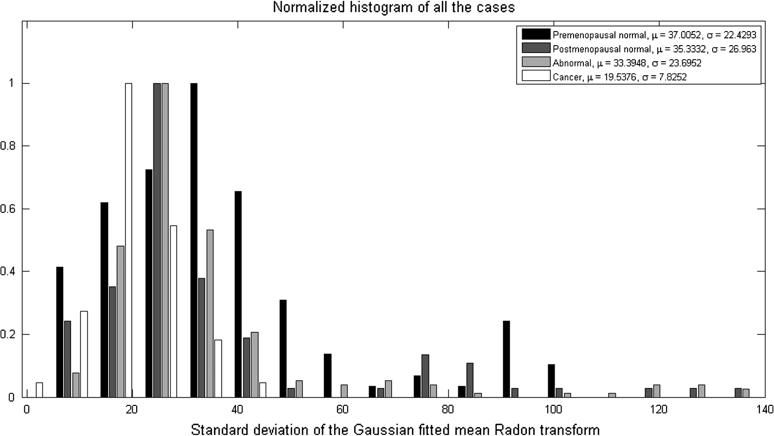 The Gaussian fitting error of the mean Radon transform had also shown a particular importance as a feature. Because the illumination is Gaussian, if the absorption from the tissue is uniform, the fitting error is small. However, if the absorption of the tissue is not uniform due to increased blood vessel activity related to tumor angiogenesis, the Gaussian shape will be disturbed and the fitting error will increase. The normalized histogram in Fig. 5 shows that the lowest fitting errors were from the postmenopausal non-cancer cases because of significantly reduced blood activity within these ovaries. Fig. 5Histograms of the fitting error showing how irregular the absorption of the ovary is from Gaussian, which could be due to random absorption distribution (cancer) or scattered vessels with higher blood activity. The postmenopausal non-cancer cases show the lowest mean fitting error because of significantly reduced blood activity in this group of patients. 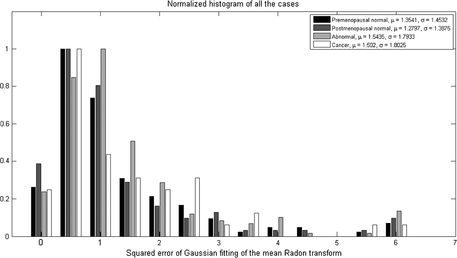 The second observation also suggests that the statistical properties of the photoacoustic images are of particular importance to account for the fluctuation of the photoacoustic intensity. The features considered for this purpose were obtained from the cropped photoacoustic images, which are the statistical variance, and the GD mean and variance over the image. Figure 6 shows the histogram of the statistical variance over the photoacoustic image for the training set. Figure 6 also shows that the optical absorption fluctuation is highest on average in the premenopausal normal ovaries because these ovaries have increased blood activity, whereas the lowest fluctuations in the absorption were on average in the cancer cases because the vasculature cluster is usually bulky with lower fluctuations. Fig. 6Histograms of the statistical variance of the photoacoustic intensity of the cropped suspicious area, which shows that the optical absorption fluctuation is the highest on average in the premenopausal normal ovaries because these ovaries have increased blood activity, whereas the lowest fluctuations in the absorption were on average in the cancer cases because the vasculature cluster is usually bulky with lower fluctuations.  In summary, an additional 9 observable features were considered, and computed for each image in the training set to train the image classifiers. 2.3.Image Classifiers TrainingThree types of classifiers were considered here, a GLM, NN, and SVM; the SVM performed the best among the three. For the GLM classifier, GLMFIT function in MATLAB was used to find the coefficients of the linear model that best follow the actual diagnosis after appropriate thresholding (zero for normal, and one for cancer case) given the training set feature values. After that, these coefficients were used with the same thresholding to compute the output of the classifier for the training set. The best training performance achieved by this classifier was 89.13% sensitivity and 85.61% specificity. A feed-forward NN was used with 6 layers; the number of neurons in each layer was chosen 104, 52, 52, 52, 13, and 1, respectively. All the transfer functions were used as TANSIG function, which is a standard thresholding function in MATLAB for NN. The training algorithm used is the resilient propagation (TRAINRP); which was found to be the best in terms of obtaining the best performance among all the other tried built-in algorithms, such as the gradient descent (TRAINGD, and TRAINGDM). However, the algorithms used can make the network extremely moody in terms of the best-achieved performance (sum of squared error). Thus, a lot of trials should be done to get the best performance. The learning algorithm used was the gradient descent with momentum (LEARNGDM); this algorithm performed the best among all the other available learning algorithms in MATLAB for our case. The trained network was used to test the same training set of images and the best performance was achieved with 86.96% true positive results (sensitivity) and 98.11% true negative results (specificity) on the training set of images. The SVM is a well-known classifier that is used in most smart cell phones for recognition of letters. SVM optimizes the separation of two populations of data by using a certain model (kernel), linear, non-linear, etc. It maps the input data into high-dimensional feature spaces and finds the hyperplane to categorize the two populations. More details on SVM can be found in Ref. 32. The SVM package in MATLAB (2008) was used with a polynomial kernel, where the sequential minimal optimization (SMO) method was used to find a hyperplane threshold that separates the cancer from non-cancer cases. The features were fed to the SVM training function, and then the trained structure was used to test back the training set of images until 100% of the images were identified correctly by the trained structure, with no false-positive or false-negative results. 3.ResultsAfter testing the training set of images and achieving the best classifiers performance, the testing set of images was evaluated. Table 2 shows a summary of the testing set of ovaries and their diagnosis. The testing images consisted of 95 images obtained from 37 ovaries of 20 patients. All were evaluated with a comprehensive test that used all the previously mentioned methods along with the three trained classifiers. For the test set, the trained SVM structure achieved the best results among the three classifiers; it was able to identify 10 of 13 cancer images correctly (sensitivity 76.92%) and 78 of 82 non-cancer images correctly (specificity 95.12%). The positive and negative predictive values were 71.43% and 96.30%, respectively.33–35 We also considered the classification by ovary whereby if one of the images from any ovary is identified by the classifier as a cancer case, then that ovary is considered a cancer case; the ovary is not considered normal unless all its images are identified as normal. Using this criterion, 4 of 4 cancer case ovaries were identified correctly (sensitivity 100%) and 29 of 33 normal ovaries were identified correctly (specificity 87.88%); Table 3 summarizes the results of all the three classifiers for the training and testing sets. Table 3Summary of the results showing the probability of error and detection, and the positive and negative predictive values based on the testing of training and non-training sets of images.
Note: PeI: False positive rate, PeII: False negative rate. It is worth noting that we tried several methods based on similarities, and linear regression analysis to reduce the number of features. However, reducing features always resulted in decreased performance of the classifier on the testing set. It was also noticed that the SVM classifier was sensitive to the selection of window size which was optimized in this study based on the actual laser illumination area. 4.SummaryWe conclude that the selected features in this study and their relation to the physiology of tumors allowed the SVM classifier to find a hyperplane threshold that gave perfect separation between 400 cancer and non-cancer images. At the same time, the trained SVM classifier was able to achieve superior sensitivity and specificity on the testing set of 95 images obtained from 37 ex vivo ovaries of 20 additional patients. These promising results will be validated in future in vivo studies. We are currently developing a real-time () coregistered ultrasound and photoacoustic imager and a dual-modality probe with a fiber assembly surrounding a commercial ultrasound transducer for in vivo ovarian cancer diagnosis. The dual modality images are coregistered with different color scales in real-time using FPGA-based reconfigurable processing technology.36,37 We made good progress overcoming challenges in adequate light delivery to tissue to achieve a reasonable photoacoustic SNR while maintaining the light energy density within the safe FDA-approved limits.38 The possible limitation of this algorithm when we apply it in in vivo transvaginal imaging would be the Gaussian illumination assumption. However, the light diffusion profile from each fiber tip inside the tissue will merge at approximately 5 mm and beyond to generate an approximate Gaussian profile to illuminate the ovarian tissue, which is more than 1-cm deep behind the vaginal muscle wall, as shown by simulations reported in Ref. 38. Additionally, our recognition algorithm proved to be robust to system changes because it performed well on the non-training data set which was obtained from a different system and ultrasound transducer than that of the training set of images. In summary, we report, to the best of our knowledge, unique features in coregistered ultrasound and photoacoustic images to allow recognition of malignant versus benign ovaries, and the hypotheses and interpretations of how these features may relate to physiology of malignant and benign ovaries. Our method has a great potential in assisting physicians in ovarian cancer diagnosis after validated by a larger patient pool in the near future. ReferencesD. A. Fishmanet al.,
“The role of ultrasound evaluation in the detection of early-stage epithelial ovarian cancer,”
Am. J. Obstet. Gynecol., 192
(4), 1214
–1222
(2005). http://dx.doi.org/10.1016/j.ajog.2005.01.041 AJOGAH 0002-9378 Google Scholar
J. TammelaS. Lele,
“New modalities in detection of recurrent ovarian cancer,”
Curr. Opin. Obstet. Gynecol., 16
(1), 5
–9
(2004). Google Scholar
V. Nossovet al.,
“The early detection of ovarian cancer: from traditional methods to proteomics. Can we really do better than serum CA-125?,”
Am. J. Obstet. Gynecol., 199
(3), 215
–223
(2008). http://dx.doi.org/10.1016/j.ajog.2008.04.009 AJOGAH 0002-9378 Google Scholar
B. V. Calsteret al.,
“Discrimination between benign and malignant adnexal masses by specialist ultrasound examination versus serum CA-125,”
J. Natl. Cancer Inst., 99
(22), 1706
–1714
(2007). http://dx.doi.org/10.1093/jnci/djm199 JNCIEQ 0027-8874 Google Scholar
M. Goozner,
“Personalizing ovarian cancer screening,”
J. Natl. Cancer. Inst., 102
(15), 1112
–1113
(2010). http://dx.doi.org/10.1093/jnci/djq296 JNCIEQ 0027-8874 Google Scholar
A. ShaabanM. Rezvani,
“Ovarian cancer: detection and radiologic staging,”
Clin. Obstet. Gynecol., 52
(1), 73
–93
(2009). http://dx.doi.org/10.1097/GRF.0b013e3181961625 COGYAK 0009-9201 Google Scholar
S. A. FuntH. Hedvig,
“Ovarian malignancies,”
Topics Magn. Res. Imag., 14
(4), 329
–337
(2003). http://dx.doi.org/10.1097/00002142-200308000-00005 TMRIEY 0899-3459 Google Scholar
R. E. Bristowet al.,
“Combined PET/CT for detecting recurrent ovarian cancer limited to retroperitoneal lymph nodes,”
Gynecol. Oncol., 99
(2), 294
–300
(2005). http://dx.doi.org/10.1016/j.ygyno.2005.06.019 GYNOA3 Google Scholar
N. Avrilet al.,
“Prediction of response to neoadjuvant chemotherapy by sequential F-18-fluorodeoxyglucose positron emission tomography in patients with advanced-stage ovarian cancer,”
J. Clin. Oncol., 23
(30), 7445
–7453
(2005). http://dx.doi.org/10.1200/JCO.2005.06.965 JCONDN 0732-183X Google Scholar
R. Kumaret al.,
“Positron emission tomography in gynecological malignancies,”
Expert Rev. Anticancer Ther., 6
(7), 1033
–1044
(2006). http://dx.doi.org/10.1586/14737140.6.7.1033 ERATBJ 1473-7140 Google Scholar
D. M. TwicklerE. Moschos,
“Ultrasound and assessment of ovarian cancer risk,”
Am. J. Roentgenol., 194
(2), 322
–329
(2010). http://dx.doi.org/10.2214/AJR.09.3562 AJROAM 0092-5381 Google Scholar
D. Timmermanet al.,
“Simple ultrasound-based rules for the diagnosis of ovarian cancer,”
Ultrasound Obstet. Gynecol., 31
(6), 681
–690
(2008). http://dx.doi.org/10.1002/uog.v31:6 0960-7692 Google Scholar
E. Fruscellaet al.,
“Sonographic features of decidualized ovarian endometriosis suspicious for malignancy,”
Ultrasound Obstet. Gynecol., 24
(5), 578
–580
(2004). http://dx.doi.org/10.1002/(ISSN)1469-0705 0960-7692 Google Scholar
R. Krugeret al.,
“Photoacoustic ultrasound (PAUS)-reconstruction tomography,”
Med. Phys., 22
(10), 1605
–1609
(1995). http://dx.doi.org/10.1118/1.597429 MPHYA6 0094-2405 Google Scholar
L. V. WangH. Wu, Biomedical Optics: Principles and Imaging, Wiley, Hoboken, NJ
(2007). Google Scholar
L. V. Wang,
“Prospects of photoacoustic tomography,”
Medical Phys., 35
(12), 5758
–5767
(2008). http://dx.doi.org/10.1118/1.3013698 MPHYA6 0094-2405 Google Scholar
X. Wanget al.,
“Noninvasive laser-induced photoacoustic tomography for structural and functional in vivo imaging of the brain,”
Nature Biotech., 21
(7), 803
–806
(2003). http://dx.doi.org/10.1038/nbt839 NABIF9 1087-0156 Google Scholar
A. OraevskyA. A. Karabutov,
“Ultimate sensitivity of time-resolved optoacoustic detection,”
Proc. SPIE, 3916
(1), 228
–239
(2000). http://dx.doi.org/10.1117/12.386326 Google Scholar
N. Weidneret al.,
“Tumor angiogenesis and metastasis: correlation in invasive breast carcinoma,”
N. Engl. J. Med., 324
(1), 1
–8
(1991). http://dx.doi.org/10.1056/NEJM199101033240101 NEJMAG 0028-4793 Google Scholar
P. VaupelF. KallinowskiP. Okunieff,
“Blood flow, oxygen and nutrient supply, and metabolic microenvironment of human tumors: a review,”
Cancer Res., 49 6449
–6465
(1989). CNREA8 0008-5472 Google Scholar
J. Gamelinet al.,
“Curved array photoacoustic tomographic system for small animal imaging,”
J. Biomed. Opt., 13
(2), 024007
(2008). http://dx.doi.org/10.1117/1.2907157 JBOPFO 1083-3668 Google Scholar
A. Aguirreet al.,
“Coregistered 3-D ultrasound and photoacoustic imaging system for ovarian tissue characterization,”
J. Biomed. Opt., 14
(5), 054014
(2009). http://dx.doi.org/10.1117/1.3233916 JBOPFO 1083-3668 Google Scholar
A. Aguirreet al.,
“Potential role of coregistered photoacoustic and ultrasound imaging in ovarian cancer detection and characterization,”
Transl. Oncol., 4
(1), 29
–37
(2010). Google Scholar
S. Srivastavaet al.,
“Automated texture-based identification of ovarian cancer in confocal microendoscope images,”
Proc. SPIE, 5701 42
–52
(2005). http://dx.doi.org/10.1117/12.590592 PSISDG 0277-786X Google Scholar
J. L. PrinceJ. M. Links, Medical Imaging Signals and Systems, 193
–195 Pearson Prentice Hall Bioengineering, Upper Saddle River, NJ
(2006). Google Scholar
B. JavidiJ. Wang,
“Optimum distortion-invariant filter for detecting a noisy distorted target in nonoverlapping background noise,”
J. OSA, 12
(12), 2604
–2614
(1995). Google Scholar
N. TowghiL. PanB. Javidi,
“Noise robustness of nonlinear filters for image recognition,”
J. Opt. Soc. Am. A, 18
(9), 2054
–2071
(2001). http://dx.doi.org/10.1364/JOSAA.18.002054 JOAOD6 0740-3232 Google Scholar
B. JavidiD. Painchaud,
“Distortion-invariant pattern recognition with fourier-plane nonlinear filters,”
Applied Opt., 35
(2), 318
–331
(1996). http://dx.doi.org/10.1364/AO.35.000318 APOPAI 0003-6935 Google Scholar
Y. A. Reyadet al.,
“Image thresholding using split and merge techniques with log-normal distribution,”
Canadian J. Image Process. Comput. Vis., 1
(3), 36
–40
(2010). Google Scholar
A. El-Zaart,
“Skin images segmentation,”
J. Comput. Sci., 6
(2), 217
–223
(2010). http://dx.doi.org/10.3844/jcssp.2010.217.223 1549-3636 Google Scholar
K.-S. Song,
“Globally convergent algorithms for estimating generalized gamma distributions in fast signal and image processing,”
IEEE Trans. Image Process., 17
(8), 1233
–1250
(2008). http://dx.doi.org/10.1109/TIP.2008.926148 IIPRE4 1057-7149 Google Scholar
N. CristianiniJ. Shawe-Taylor, An Introduction to Support Vector Machines and Other Kernel-Based Learning Methods, Cambridge University Press, Cambridge, UK
(2000). Google Scholar
A. Papoulis, Probability, Random Variables, and Stochastic Processes, 4th ed.McGraw-Hill, New York
(2002). Google Scholar
Y. Bar-ShalomX. Rong LiT. Kirubarajan, Estimation with Applications to Tracking and Navigation, John Wiley & Sons, New York
(2001). Google Scholar
R. K. GunnarssonJ. Lanke,
“The predictive value of microbiologic diagnostic tests if asymptomatic carriers are present,”
Stat. Med., 21
(12), 1773
–1785
(2002). http://dx.doi.org/10.1002/(ISSN)1097-0258 SMEDDA 1097-0258 Google Scholar
U. Alqasemiet al.,
“FPGA-based reconfigurable processor for ultra fast interlaced ultrasound and photoacoustic imaging,”
IEEE Trans. Ultrason. Ferroelectrics Freq. Contr., 59
(7), 1344
–1353
(2012). http://dx.doi.org/10.1109/TUFFC.2012.2335 Google Scholar
U. Alqasemiet al.,
“Ultra fast ultrasound and photoacoustic coregistered imaging system based on FPGA parallel processing,”
Proc. SPIE, 8223 82232U
(2012). http://dx.doi.org/10.1117/12.907583 PSISDG 0277-786X Google Scholar
P. Kumavoret al.,
“Demonstration of a coregistered pulse-echo/photoacoustic probe for real time in vivo imaging of ovarian tissue,”
J. Biomed. Opt.,
(2012). JBOPFO 1083-3668 Google Scholar
|
|||||||||||||||||||||||||||||||||||||||||||||||||||||||||||||||||||||||||||||||||||||||||||||||||||||||||||||||||||||||||||||||||||||||||||||||||||||||||||||||||||||||||||||||||||||||||||||||||||||||||||||||||||||||||||||||||||||||||||||||||||||||||||||||||||||||||||||||||||||||||


