|
|
1.IntroductionMolecular imaging (MI), emerging as an indispensable research tool, enhances the understanding of the physiological and pathological changes in organisms. This noninvasive technology is capable of visualizing the dynamic molecular and cellular processes taking place in vivo over a period of time; while the conventional route known as the gold standard is to perform a biopsy before the tissue is observed at a certain time. Hence the development of MI is of growing significance for early intervention of disease, especially for cancer, which has a global increase in incidence rate.1–3 There are different modalities of MI, and each modality has its own advantages, mainly varying in image resolution, detection depth, molecular sensitivity, available probes, and equipment cost.4 The common modalities—including ultrasound imaging, computed tomography (CT), and magnetic resonance imaging (MRI)—are generally good at detecting a lesion larger than 1 cm in diameter,5 while every cubic centimeter of the tumor contains approximately 0.5 to 3 billion cancer cells, which is basically too late for early detection. Thus, new imaging methods and medical equipment adapted to detect minute tumors still need to be developed. The existing literature on multimodal fusion suggests new opportunity.6–8 Hereby, dual-modality tomography (DMT) has been utilized in this study, which provides multiview bioluminescence imaging (BLI) and microcomputed tomography (μCT). BLI, one of the major modalities in optical molecular imaging, reflects the functional information by collecting the luminescent signal emitted from the internal tumor cells expressing bioluminescent proteins. Together with the anatomical structures generated by μCT, DMT enables localization of the tumor region in three-dimensional (3-D), as well as performing a quantitative analysis. By combining the two imaging modalities, DMT therefore brings together the merits of good sensitivity, high resolution, fast speed, and low instrumentation cost, potentially making it possible for detecting liver cancer at an early stage. Since the classical imaging techniques usually depend on observing the physical properties of the tissues during diagnosis, they could hardly reveal the cellular or molecular changes associated with disease until when some obvious morphological changes occur in the lesion areas. In contrast, DMT provides higher detection sensitivity and more precise tumor localization due to the following three reasons.
For hybrid optical/μCT imaging, it is the 3-D reconstruction of the dual-modality data that is challenging.9 Reconstruction mainly refers to the procedure of creating the object in 3-D from a set of planar images, and usually a precise reconstruction result is the essential premise for the subsequent steps in image processing. In particular, DMT reconstruction involves an ill-posed inverse problem for the reason that the available information of the surface photon density is more limited than the unknown internal bioluminescence intensity, which is also regarded as an underdetermined system of linear equations. Moreover, the numerical computation of reconstruction could be time-consuming due to the large scale of three-dimensional dual-modality data, and it usually depends on selecting reconstruction parameters. Over the past few years, the related work aiming at solving the above challenging problems has been extensively developed. To alleviate the ill-posedness and ensure reconstruction reliability, the multispectral algorithm was introduced to increase the independent boundary measurements,10 while the permissible source region approach was demonstrated to reduce the number of the unknowns.11 To improve the reconstruction accuracy, classical Newton’s methods with Tikhonov regularization were widely used,12–14 while they performed computationally costly to guarantee the convergence of the solution. To enhance the reconstruction efficiency, the graph cuts based methods were organized to conserve computation time due to the gradient-free optimization.15,16 Although the reconstruction approaches usually work well in some specific and highly controlled situations, no efforts need to be spared in investigating more general cases.17 In this paper, a parallel iterative shrinkage algorithm has been demonstrated for the dual-modality tomography, i.e., the hybrid optical/μCT imaging. This method has implemented the detection and visualization of the mouse liver tumors at an early stage, enabling lesion localization and its quantitative analysis. In Sec. 2, the photon diffusion model will be described mathematically, and then the principle and features of the PIS method will be introduced in detail. In Sec. 3, the feasibility and limitations of the PIS method for DMT will be thoroughly assessed, followed by the 3-D reconstruction results of the two in vivo experiments on mice. In Sec. 4, the conclusion and the future plan for this work will be summarized. 2.MethodsIn order to compute the 3-D distributions of the lesion regions in mice, the following four steps were essentially taken to process the raw data in multiple views acquired by the DMT system. Figure 1 gives an overview of the whole procedure.
Fig. 1The method overview. First, pre-process the raw data with segmentation, discretization, and registration; then, set up the photon diffusion model and conduct the PIS reconstruction to localize the luminescent source representing the tumor region; finally, visualize the reconstruction results in 3-D and do the necessary analysis.  2.1.Photon Diffusion ModelThe photon diffusion model describes the propagation of light through the mouse. In optical imaging, the luminescent source in the near infrared range (NIR) has low energy, leading to a diffusion-dominant transport process in a turbid medium such as biological tissues. For this reason, the particle properties of light are mainly taken into account, including scattering and absorption; the wave nature such as polarization and interference are neglected.18 Based on those premises, the light propagation is modeled by a diffusion approximation with the Robin boundary condition. The diffusion equation is adapted to characterize the propagation in biological tissues with the optical properties of high scattering and low absorption. It is the first-order spherical harmonics approximation for the radiative transfer equation,19 which can be written as Eq. (1) in the steady-state domain. where is the diffusion coefficient, and ; is the absorption coefficient; is the anisotropy parameter; is the scattering coefficient; is a position vector; is the photon flux density; is the signal source distribution; is the region of biological tissues.The Robin boundary condition is employed due to the completely dark imaging environment of BLI20 without any external photons, which is defined as where is the boundary mismatch factor between the biological tissues and air, and ; is the refractive index of the biological tissues; is the unit outward normal on ; is the boundary of the biological tissues.According to the Robin boundary condition, the theoretical outgoing photon density on the surface of the mouse is calculated by where is the theoretical value of the outgoing photon density on the surface.After applying the finite element method based on the variation principle to Eqs. (1) and (2), the linear relationship can be built between the measured outgoing photon density on the surface and the bioluminescence intensity inside the body via replacing the variables with the matrix-vector forms:20 where is the system matrix, standing for the optical properties of the biological tissues; is the measured outgoing photon density on the surface.In Eq. (4), the photon density on surface can be calculated from the multiview optical images captured by a cooled charge-coupled device. Each element of the system matrix can be gained by Refs. 19 and 21: where is the basis function in the finite element method.Hence the procedure to solve the diffusion equation has been simplified into the form of a linear function, which can improve computational efficiency. It is peculiarly worth mentioning that Eq. (4) is an underdetermined system of linear equations with fewer equations than unknowns. This is because the available information of the surface photon density is far more limited than the unknown internal bioluminescence intensity, consequently causing difficulties in the following 3-D reconstruction. 2.2.Prior Knowledge and Optimal StrategyThe DMT reconstruction is involved in solving an undetermined system of linear equations, which is mathematically considered to be an ill-posed problem on account of its infinite solutions. In order to reduce the ill-posedness, a priori knowledge known as a sparse constraint is introduced, by which an approximation close to the exact solution can be eventually found. Since this paper emphasizes the detection of early-stage tumors, there usually turns out to be sparse signals in the biological organism,22 referring to a distribution with a large number of zeros except for minimal support of the solution space that denotes the lesion areas. Thus the methods for sparse signals recovery (SSR) offer valuable alternatives to DMT reconstruction. The essence of SSR is to utilize the limited linear observations via a normal optimal strategy. Since the samples required by SSR could be less than the quantity needed by the Nyquist sampling theorem, the underdetermined system of equations can be solved by finding the best basis that stands for the bioluminescence intensity. A number of iterative algorithms,23–27 which have been developed to retrieve sparse signals include the Born iterative method, Truncate-Newton, Levenberg-Marquardt approach, etc. Furthermore, a regularization strategy was also exploited for DMT reconstruction. Generally, the simplest solution to Eq. (4) is in the form of the least square expressed as Eq. (6), but it tends to amplify the errors generated by noise. In order to make the reconstruction more practical, a constraint condition known as a regularization term is added. For instance, one of the most commonly used methods named Tikhonov regularization considers the norms constraint for the unknown internal source,28 the form of which is written in Eq. (7). Although this method can optimize the results, it still leads to the over-smooth problem, which blurs the reconstructed source boundary and misses part of the source information. where is the regularization parameter.To overcome the above difficulties, we incorporated the sparse signals as the prior knowledge and used a more generalized form for the constraint condition, the norm regularization term, shown in Eq. (8). So far, the optimal object function for retrieving the DMT signals has been obtained, which is a linear inverse problem formulated as Eq. (9). The internal source distribution representing the tumor region can be ultimately determined by solving the object function via optimal minimization in the next section. where stands for the norm; stands for the norm; is a real number in the range from one to two.2.3.Parallel Iterative Shrinkage AlgorithmThe iterative shrinkage strategy is a newly emerged numerical computational method. It surpasses the traditional iteration optimization such as the steepest-descent, the conjugate gradient and the interior-point29–31 in terms of temporal and spatial efficiency particularly when solving the multidimension problem. Because of those strengths, the iterative shrinkage methods have recently been applied to image denoising and the inverse problem.32 The PIS approach, belonging to the iterative shrinkage methods,33 intrinsically converts a complex process of optimizing the multidimension function into a set of parallel one-dimension optimizations with respect to each variable. In other words, the full set of unknown variables is iteratively optimized at the same time instead of being updated sequentially, by which the computational complexity can thereby be simplified. To further illustrate how such an algorithm fits into DMT reconstruction, we mathematically derived the PIS method using the following four steps.
In summary, the PIS algorithm for the DMT reconstruction can be concisely demonstrated by the flowchart in Fig. 3. 3.Results and DiscussionTo validate the feasibility of the PIS method for the DMT reconstruction, an in vivo experiment on the nude mouse that was implanted with a plastic luminescent bead in the liver has been conducted using the hybrid optical/μCT imaging system developed by our group.34 Then we have applied the proposed approach to another in vivo experiment on an HCCLM3 orthotopic xenograft mouse model. Note that HCCLM3 stands for a human hepatocellular carcinoma cell line with high metastatic potential. 3.1.Dual-Modality Imaging System SetupThe DMT system, surrounded in a completely dark environment, provides two modalities: multiview BLT and μCT. The schematic illustration of the system is given by Fig. 4, which is mainly equipped with a cooled CCD, a set of optical lenses, an x-ray generator, an x-ray detector, and a rotating stage (the manufacturers and models are listed in Table 1). This system enables noninvasive in vivo imaging for small animals, making it possible to observe the dynamic biological behavior in real time. However, if detecting the same activity taking place in the body by the conventional method, a group of experimental mice have to be sacrificed for the inevitable pathological section analysis. Besides reducing the quantity of the experimental animals, this new hybrid imaging method can also result in more reliable datasets since the whole dynamic procedure can be achieved on the same mouse, thus avoiding individual differences. Fig. 4The schematic illustration of the DMT system. It provides multiview BLI and μCT, the major devices of which are illustrated in Table 1.  Table 1The manufacturers and models for the components of the DMT system.
3.2.Data Acquisition and Image PreprocessingPrior to the experiment, the dual-modality raw data was collected, respectively. The acquisition time for the entire procedure was within 10 min, which could be tolerated by the mice. As delineated in Fig. 4, the mouse was firstly placed on the automatic rotating stage. Afterward, the photons emitted from the mouse body were captured in four different views by the cooled CCD. The four planar optical images are displayed in Fig. 5. At last, the cone-beam μCT projection data with 360-deg views was scanned using the x-ray generator and the detector. Fig. 5The multi-view BLI data of the experimental nude mouse with an implanted luminescent bead. Four pictures taken at 0 deg, 90 deg, 180 deg, and 270 deg by the cooled CCD.  After achieving the raw data, some necessary preprocessing operations were carried out to make the data suitable for posterior reconstruction.
Fig. 6The heterogeneous volume data and the surface photon distribution of the experimental nude mouse with an implanted luminescent bead. (a) The volume data of the heterogeneous mouse model after the segmentation of the major organs and tissues including the heart, lungs, liver, muscle, and skeleton; (b) the surface photon distribution of the mouse body after registration, where the photons are assembled as a bright spot on the bottom left. Compared with (a), it could be estimated that the spot is close to or located exactly at the liver region.  3.3.In Vivo Experiment on the Bead-Implanted MouseThe experimental nude mouse’s liver in this section was surgically implanted with the luminescent bead. Anterior to imaging, the mouse was injected through the caudal tail vein with 0.3-ml Fenestra vascular contrast agent to enhance the μCT images, followed by 0.3 ml of anesthetic at a concentration via intraperitoneal injection. When the anesthetic set in, an irregular-shaped bead the size of was embedded into the mouse. This luminescent source was suited for stimulating the liver tumor inside the living organism, because its wavelength ranged from 650 to 700 nm, which is identical to that of the light produced by firefly luciferase. It is worth mentioning that this study could examine the reconstruction accuracy of the PIS method, because the luminescent bead was wrapped in a plastic material, which could be easily detected by μCT. After acquiring the raw data using the DMT system, the μCT data was reconstructed into the volume data, three slices of which are shown in Fig. 7, where the square marks the location of the luminescent bead at the coordinate (24.6, 20.0, 7.2). After combining the optical data displayed in Fig. 5, the heterogeneous volume and the surface photon distribution shown in Fig. 6 could be therefore achieved. To distinguish the different optical properties of the organs and tissues, the adding-doubling technique36 was utilized to improve the heterogeneous mouse model, where the organs and tissues were assigned the corresponding coefficients of absorption and scattering in Table 2. Finally, the reconstruction based on the PIS method was performed to localize where the luminescent bead was inside the mouse body. The reconstruction results will be evaluated in more detail in the next section. Fig. 7Three slices of the μCT data, where the yellow square marks the location of the luminescent bead: (a) the coronal view; (b) the sagittal view; (c) the transversal view.  Table 2The optical properties of the mouse organs and tissues (mm−1), where the first row represents the absorption coefficient, while the second row denotes the scattering coefficient.
3.4.Evaluation of Reconstruction AccuracyTo validate the reconstruction accuracy of the PIS approach, comparisons were made between the reconstructed internal source and the plastic luminescent bead. Figure 8 gives the results in the case when and , demonstrating the size of the reconstructed source and its location to the organs and tissues inside the mouse body. Fig. 8The reconstruction results using the PIS method in the case when and : (a) the front view in 3-D; (b) the side view in 3-D while setting the liver region as invisible; (c) the coronal view of the μCT slice where the center of the luminescent bead was located; (d) the sectional view of the DMT reconstruction results where the reconstructed internal source was located; (e) the corresponding iterative curve, reflecting the convergence speed of the reconstruction.  It can be seen from Fig. 8(a) that the reconstructed source is located in the liver region, and the coordinate of the source center is (24.0, 19.8, 7.4). To display the entire source more clearly, the liver was concealed in Fig. 8(b), enabling the measurement of the source size, which was . In addition, Fig. 8(c) shows the sectional view of the μCT slice where the center of the luminescent bead was located, which was visually in good agreement with the center of the reconstructed source shown in Fig. 8(d). A further computation confirmed that the position bias between the two centers was approximately 0.66 mm. The above results suggest the lesion region was less than 3 mm in diameter but could be detected by means of the PIS method, with a position bias no more than 1 mm. 3.5.Evaluation of Reconstruction EfficiencyTo examine the reconstruction efficiency of the PIS algorithm, take the same case as an example. Figure 8(e) describes the convergence speed of the iterative reconstruction with the same parameters mentioned in the former section. It is noted that the iterative curves still resemble each other even when the parameters are changed. During the total 40 iterations, the value of the optimal object function decreased substantially, moving towards an ultimate convergence. The whole procedure of this reconstruction cost 9.82 s. In particular, the value tended to be zero as early as the 20th iteration, and then it became more stable. Moreover, the classical Newton’s algorithm and the generalized graph cut (GGC) approach were also applied to reconstruct the same dataset.37 The comparison of the reconstruction efficiency was made based on the data in Table 3. It shows the time consumed by the two different methods as well as the proposed one for reconstructing the four groups of datasets whose sizes are determined by the density of the discrete volumetric mesh. Table 3The comparison of the reconstruction efficiency based on different methods. The size of the volumetric mesh equals the number of nodes multiplied by the number of tetrahedral elements.
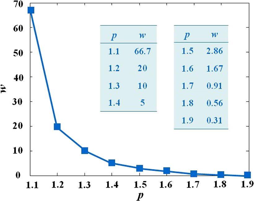
The results reveal that: 1. When reconstructing the same dataset, the GGC approach works more efficiently than Newton’s algorithm, but is less efficient than the proposed PIS method; 2. When the size of the dataset increases, the PIS method becomes more computationally competitive; 3. all of the datasets are discretized based on the whole mouse torso, which means the proposed method is not only time efficient, but also has the potential for practical applications. 3.6.Evaluation of Reconstruction ReliabilityTo verify the reconstruction reliability of the PIS method, we have conducted 180 reconstructions for testing its tolerance with different parameters. Generally speaking, the reconstruction accuracy is considerably affected by the regularization parameter and the norm, where slight changes may dramatically have an impact on the results. In this section, the regularization parameter was selected with different orders of magnitude, with ranging from 1 to 20; as for the norm, was chosen to be between 1.1 and 1.9. The sectional views of the reconstruction results are partly delineated in Figs. 9 and 10. Fig. 9The comparisons of the reconstruction results in sectional views with different regularization parameters : (a) the coronal view of the μCT slice where the center of the luminescent bead was located; (b) to (j) the sectional views of the reconstruction results in the cases when , , , , , , , , , respectively, while maintaining the same value, .  Fig. 10The comparisons of the reconstruction results in sectional views with a different norm: (a) the coronal view of the μCT slice where the center of the luminescent bead was located; (b) to (j) the sectional views of the reconstruction results in cases when , 1.2, 1.3, 1.4, 1.5, 1.6, 1.7, 1.8, 1.9, respectively, while maintaining the same value, .  Comparing the locations between the luminescent bead in Fig. 9(a) and the reconstructed bright spots in Fig. 9(b) to 9(j), we found that they were visually in good agreement by virtue of the auxiliary grid. Further computation revealed that the position bias in each reconstruction was less than 1 mm, and more details have been explored about the position bias. 1. It reaches the lowest peak when ; 2. it maintains a smaller value when , ensuring satisfying results; 3. it rises substantially when , meaning undesirable options. Therefore the proposed algorithm is robust to a wide variety of parameters, whereas the regularization parameter could be no more than , and the norm has a more flexible selection. 3.7.In Vivo Experiment on HCCLM3 Orthotopic Xenograft Mouse ModelUnlike the experimental mouse introduced in Sec. 3.3, the nude mouse in this section was an orthotopic xenograft model inoculated with HCCLM3 cell lines. Those fLuc-expressing HCCLM3 cell lines are suitable for BLI. Before imaging, both the anesthetic and luciferine were successively injected into the mouse, where the photons were emitted during the oxidation reaction on the condition that luciferase met luciferine. The amount of the outgoing photons collected by the DMT system is linearly correlated to the quantity of the liver cancer cells inside the mouse, because the chemical reaction will occur only when the cancer cells are alive, and only one photon will be sent out every time when the reaction works. During imaging, the optical images in the four views were attained by the BLI modality, and the volume data at 360 deg was scanned by the μCT modality. The accumulated acquisition time was about 7 min in total, in which each optical image took 10 s of the integral time while the μCT scanning cost 60 s. The raw optical pictures in Fig. 11 describe the photon distribution in two-dimensional (2-D) of the whole mouse, where two bright spots could be caught from 0 deg and 90 deg, but not from obviously visible luminescence at 180 deg and 270 deg. After imaging, the mouse was subjected to laparotomy and was analyzed using H&E staining, and lesions could be observed in the liver region. Fig. 11The multi-view BLI data of the HCCLM3 orthotopic xenograft mouse model. Four pictures take at 0 deg, 90 deg, 180 deg, and 270 deg via the cooled CCD.  Prior to reconstruction, the dual-modality data was preprocessed. After segmentation, the μCT volume of the whole mouse is shown in Fig. 12(a), which clearly depicts the anatomical structure in 3-D, but the tumor could be hardly observed due to the limitations of μCT, such as the low contrast for detecting soft tissues. After registration, the 2-D photon distribution was mapped onto the surface of the 3-D volume data. From Fig. 12(b), we can notice that there are two bright spots on the surface of the mouse abdomen, consisting of the gathered photons emitted from the internal liver tumors, but it could neither offer the 3-D distribution of the internal tumors, nor suggest how they were located in relation to the organs and tissues inside the mouse’s body. That is why the following reconstruction based on the PIS approach is essential. Fig. 12The heterogeneous volume data and the surface photon distribution of the HCCLM3 orthotopic xenograft mouse model: (a) the volume data of the heterogeneous mouse model after the segmentation of the major organs and tissues including the heart, lungs, liver, muscle, and skeleton; (b) the surface photon distribution of the mouse body after registration.  When the reconstruction was performed, the whole mouse volume data was discretized into a volumetric mesh containing 5193 nodes and 53,653 tetrahedral elements. Figure 13 describes the results in the case when and , where the reconstruction time is 9.83 s. The liver region is set to be invisible in order to not cover the reconstructed tumors, and it can be perceived that there are two tumors inside the mouse’s body. The smaller one measures about , and the volume of the larger one is around . Fig. 13The reconstruction results of the HCCLM3 orthotopic xenograft mouse model using the PIS method in case when and , including a front view and two side views.  The above findings suggest that the PIS method is able to detect the lesions in the above biomedical application, and two liver tumors have been localized at the same time in the HCCLM3 orthotopic xenograft mouse model. 4.Conclusions and Future WorkThe PIS reconstruction algorithm proposed in this research project is capable of enhancing accuracy efficiency, and reliability in whole-body liver cancer detection mainly using the following three strategies:
In addition, two in vivo experiments on nude mice have been conducted to evaluate the feasibility and limitations of the proposed method in liver cancer detection. The results indicate that:
Future work will emphasize on improving the drawbacks of the proposed PIS algorithm. Despite tumor size, which could only be measured approximately, it is still difficult in achieving an accurate tumor boundary, which is critically important for surgical removal. This is because FEM was employed to establish the photon diffusion model in this study, and it is fundamentally limited in describing the shape of objects. On the other hand, the second experiment could be extended further. It deserves more in-depth studies of the weak signals from the internal cancer cells, as well as tumor metastasis resulting in more internal luminescent sources instead of only one or two, so that the whole-body reconstruction for multisource mouse model can be done better. AcknowledgmentsThis study was supported by the National Basic Research Program of China (973 Program) under Grant No. 2011CB707700, the Knowledge Innovation Project of the Chinese Academy of Sciences under Grant No. KGCX2-YW-907, the National Natural Science Foundation of China under Grant Nos. 81227901, 61231004, 81027002, 81261120414, the Chinese Academy of Sciences Visiting Professorship for Senior International Scientists under Grant No. 2012T1G0036, and the Beijing Natural Science Foundation No. 4111004. ReferencesR. WeisslederJ. M. Pittet,
“Imaging in the era of molecular oncology,”
Nature, 452
(7187), 580
–589
(2008). http://dx.doi.org/10.1038/nature06917 NATUAS 0028-0836 Google Scholar
A. MorabiaT. Abel,
“The WHO report ‘Preventing chronic diseases: a vital investment’ and us,”
Soz Praventivmed., 51
(2), 74
–74
(2006). http://dx.doi.org/10.1007/s00038-005-0015-7 Google Scholar
A. Jemalet al.,
“Global cancer statistics,”
CA: A Cancer J. Clin., 61
(2), 69
–90
(2011). http://dx.doi.org/10.3322/caac.v61:2 1542-4863 Google Scholar
T. F. MassoudS. S. Gambhir,
“Molecular imaging in living subjects: seeing fundamental biological processes in a new light,”
Genes Dev., 17
(5), 545
–580
(2003). http://dx.doi.org/10.1101/gad.1047403 GEDEEP 0890-9369 Google Scholar
A. Muhiet al.,
“Diagnosis of colorectal hepatic metastases: comparison of contrast-enhanced CT, contrast-enhanced US, superparamagnetic iron oxide-enhanced MRI, and gadoxetic acid-enhanced MRI,”
J Magn. Reson. Imaging, 34
(2), 326
–335
(2011). http://dx.doi.org/10.1002/jmri.v34.2 1053-1807 Google Scholar
H. Fan-Minogueet al.,
“Noninvasive molecular imaging of c-Myc activation in living mice,”
Proc Natl. Acad. Sci., 107
(36), 15892
–15897
(2010). http://dx.doi.org/10.1073/pnas.1007443107 PNASA6 0027-8424 Google Scholar
M. Nahrendorfet al.,
“Hybrid PET-optical imaging using targeted probes,”
Proc Natl. Acad. Sci., 107
(17), 7910
–7915
(2010). http://dx.doi.org/10.1073/pnas.0915163107 PNASA6 0027-8424 Google Scholar
A. Aleet al.,
“FMT-XCT: in vivo animal studies with hybrid fluorescence molecular tomography-X-ray computed tomography,”
Nat. Methods, 9
(6), 615
–620
(2012). http://dx.doi.org/10.1038/nmeth.2014 1548-7091 Google Scholar
V. Ntziachristos,
“Going deeper than microscopy: the optical imaging frontier in biology,”
Nat. Methods, 7
(8), 603
–614
(2010). http://dx.doi.org/10.1038/nmeth.1483 1548-7091 Google Scholar
C. Kuoet al.,
“Three-dimensional reconstruction of in vivo bioluminescent sources based on multispectral imaging,”
J. Biomed. Opt., 12
(2), 024007
(2007). http://dx.doi.org/10.1117/1.2717898 JBOPFO 1083-3668 Google Scholar
Y. Luet al.,
“A multilevel adaptive finite element algorithm for bioluminescence tomography,”
Opt. Express, 14
(18), 8211
–8223
(2006). http://dx.doi.org/10.1364/OE.14.008211 OPEXFF 1094-4087 Google Scholar
J. Tianet al.,
“Multimodality molecular imaging—improving image quality,”
IEEE Eng. Med. Biol. Mag., 27
(5), 48
–57
(2008). http://dx.doi.org/10.1109/MEMB.2008.923962 IEMBDE 0739-5175 Google Scholar
Y. Luet al.,
“Source reconstruction for spectrally-resolved bioluminescence tomography with sparse a priori information,”
Opt. Express, 17
(10), 8062
–8080
(2009). http://dx.doi.org/10.1364/OE.17.008062 OPEXFF 1094-4087 Google Scholar
G. Wanget al.,
“In vivo mouse studies with bioluminescence tomography,”
Opt. Express, 14
(17), 7801
–7809
(2006). http://dx.doi.org/10.1364/OE.14.007801 OPEXFF 1094-4087 Google Scholar
K. Liuet al.,
“A fast bioluminescent source localization method based on generalized graph cuts with mouse model validation,”
Opt. Express, 18
(4), 3732
–3745
(2010). http://dx.doi.org/10.1364/OE.18.003732 OPEXFF 1094-4087 Google Scholar
P. RodríguezB. Wohlberg,
“Efficient minimization method for a generalized total variation functional,”
IEEE Trans. Image Process., 18
(2), 322
–332
(2009). http://dx.doi.org/10.1109/TIP.2008.2008420 IIPRE4 1057-7149 Google Scholar
N. Blow,
“In vivo molecular imaging: the inside job,”
Nat. Methods, 6
(6), 465
–469
(2009). http://dx.doi.org/10.1038/nmeth0609-465 1548-7091 Google Scholar
L. V. WangH. I. Wu, Bio Opt: Principles and Imaging, John Wiley and Sons, Hoboken
(2007). Google Scholar
W. X. Conget al.,
“Practical reconstruction method for bioluminescence tomography,”
Opt. Express, 13
(18), 6756
–6771
(2005). http://dx.doi.org/10.1364/OPEX.13.006756 OPEXFF 1094-4087 Google Scholar
S. R. Arridge,
“Optical tomography in medical image,”
Inverse Problm., 15
(2), R41
–R93
(1999). http://dx.doi.org/10.1088/0266-5611/15/2/022 INPEEY 0266-5611 Google Scholar
M. Schweigeret al.,
“The finite element method for the propagation of light in scattering media: boundary and source conditions,”
Med. Phys., 22
(11), 1779
–1792
(1995). http://dx.doi.org/10.1118/1.597634 MPHYA6 0094-2405 Google Scholar
S. S. ChenD. L. DonohoM. A. Saunders,
“Atomic decomposition by basis pursuit,”
SIAM J. Sci. Comput., 20
(1), 33
–61
(1998). http://dx.doi.org/10.1137/S1064827596304010 SJOCE3 1064-8275 Google Scholar
J. C. Yeet al.,
“Modified distorted Born iterative method with an approximate Frechet derivative for optical diffusion tomography,”
J. Opt. Soc. Amer., 16
(7), 1814
–1826
(1999). http://dx.doi.org/10.1364/JOSAA.16.001814 JOAOD6 1084-7529 Google Scholar
Y. Q. Yaoet al.,
“Frequency-domain optical imaging of absorption and scattering distributions by a born iterative method,”
J Opt. Soc. Amer., 14
(1), 325
–342
(1997). http://dx.doi.org/10.1364/JOSAA.14.000325 JOAOD6 1084-7529 Google Scholar
R. RoyE. Sevick-Muraca,
“Truncated newton’s optimization scheme for absorption and fluorescence optical tomography: part I theory and formulation,”
Opt. Express, 4
(10), 353
–371
(1999). http://dx.doi.org/10.1364/OE.4.000353 OPEXFF 1094-4087 Google Scholar
M. SchweigerS. R. ArridgeD. T. Delpy,
“Application of the finite-element method for the forward and inverse models in optical tomography,”
J. Math. Imaging Vis., 3
(3), 263
–283
(1993). http://dx.doi.org/10.1007/BF01248356 JIMVEC 0924-9907 Google Scholar
K. D. PaulsenH. B. Jiang,
“Enhanced frequency-domain optical image reconstruction in tissues through total-variation minimization,”
Appl. Opt., 35
(19), 3447
–3458
(1996). http://dx.doi.org/10.1364/AO.35.003447 APOPAI 0003-6935 Google Scholar
B. KaltenbacherA. KirchnerB. Vexler,
“Adaptive discretizations for the choice of a Tikhonov regularization parameter in nonlinear inverse problems,”
Inverse Problm., 27
(12), 125008
(2011). http://dx.doi.org/10.1088/0266-5611/27/12/125008 INPEEY 0266-5611 Google Scholar
C. E. ChidumeC. O. ChidumeB. Ali,
“Convergence of hybrid steepest descent method for variational inequalities in Banach spaces,”
Appl. Math. Comput., 217
(23), 9499
–9507
(2011). http://dx.doi.org/10.1016/j.amc.2011.02.099 AMHCBQ 0096-3003 Google Scholar
Z. StrakosP. Tichy,
“On error estimation in the conjugate gradient method and why it works in finite precision computations,”
Electron. Trans. Numer. Anal., 13 56
–80
(2002). 1068-9613 Google Scholar
M. RojasT. Steihaug,
“An interior-point trust-region-based method for large-scale non-negative regularization,”
Inverse Problm., 18
(5), 1291
–1307
(2002). http://dx.doi.org/10.1088/0266-5611/18/5/305 INPEEY 0266-5611 Google Scholar
J. L. StarckE. J. CandesD. L. Donoho,
“The curvelet transform for image denoising,”
IEEE Trans. Image Process., 11
(6), 670
–684
(2002). http://dx.doi.org/10.1109/TIP.2002.1014998 IIPRE4 1057-7149 Google Scholar
M. Elad,
“Why simple shrinkage is still relevant for redundant representations,”
IEEE Trans. Inform. Theor., 52
(12), 5559
–5569
(2006). http://dx.doi.org/10.1109/TIT.2006.885522 IETTAW 0018-9448 Google Scholar
S. P. Zhuet al.,
“Cone beam micro-CT system for small animal imaging and performance evaluation,”
Int. J. Biomed. Imaging, 2009
(2009), 960573
(2009). http://dx.doi.org/10.1155/2009/960573 1687-4188 Google Scholar
G. R. Yanet al.,
“Fast cone-beam CT image reconstruction using GPU hardware,”
J. X-Ray Sci. Technol., 16
(4), 225
–234
(2008). JXSTE5 0895-3996 Google Scholar
S. A. PrahlV. GemertA. J. Welch,
“Determining the optical properties of turbid media by using the adding doubling method,”
Appl. Opt., 32
(4), 559
–568
(1993). http://dx.doi.org/10.1364/AO.32.000559 APOPAI 0003-6935 Google Scholar
K. Liuet al.,
“Tomographic bioluminescence imaging reconstruction via a dynamically-sparse regularized global method in mouse models,”
J. Biomed. Opt., 16
(4), 046016
(2011). http://dx.doi.org/10.1117/1.3570828 JBOPFO 1083-3668 Google Scholar
|