
|
|
1.IntroductionLaser speckle contrast imaging (LSCI) is an optical imaging technique that has classically been used to study blood flow changes in neurophysiology studies.1,2 In addition, LSCI has been shown to produce high-resolution and high-contrast images of cerebral microvascular morphology by exploiting the temporal processing scheme.3 As a technique for imaging cerebral microvessels, LSCI offers distinct advantages over concurrent optical methods. First, LSCI is a full-field technique and thus can visualize microvessels over a wide field of view (FOV) as large as , allowing a holistic picture of proximal and distal regions. Second, LSCI derives its contrast intrinsically from the flow of red blood cells inside blood vessels, thereby not requiring any externally injected contrast agents. Third, LSCI can monitor vasculature through a thinned skull preparation in rats; that is, without mechanically or chemically perturbing the brain. In addition to the high spatial resolution, LSCI can infer blood flow within microvessels.4 These advantages make LSCI a prime candidate for longitudinal imaging of microvasculature. Consequently, in this paper, we investigate the suitability of LSCI for monitoring through the thinned skull the microvascular remodeling that accompanies the progression of an intracranial tumor. Therapeutic inhibition of new vessel formation reserves the potential to arrest tumor growth. This idea has made tumor angiogenesis a widely researched topic.5–7 Current methods of imaging angiogenesis are limited in their scope and capability.8 The most commonly used noninvasive methods of imaging tumor angiogenesis, namely, x-ray angiography,9 magnetic resonance imaging (MRI),10 computed tomography (CT),11 and positron emission tomography (PET),12 have poor spatial resolution and produce images of angiogenic regions rather than angiogenic vessels.13 These techniques are generally used in conjunction with the intra-vascular introduction of a contrast agent and are therefore unsuitable for repeated, long-term monitoring. The laboratory gold standard for imaging microvascular architecture is vascular casting.14,15 However, this technique requires sacrificing the animal, which makes it impossible to conduct longitudinal studies in a single animal or to monitor blood flow in vivo. Fluorescent labeling16 and immunohistochemical techniques17 suffer the same disadvantage. Optical imaging techniques generally rely on contrast enhancement using fluorescent dyes to obtain high-resolution images. Since tumor vessels are inherently leaky, dye leakage can help identify tumor angiogenesis but simultaneously contaminate the FOV.18 Thus, even high-resolution techniques such as multiphoton imaging suffer loss of vascular contrast in tumor environments due to dye extravasation.19 Optical coherence tomography (OCT) has also been used for tumor detection, but tumor classification has been made on the basis of optical properties of tumor cells.20 Vakoc et al. have recently acquired state of the art in vivo images of the tumor microenvironment using optical frequency domain imaging, an advanced form of OCT.21 While OCT can provide good depth resolution, the in-plane images produced by OCT are difficult to interpret22 and could be complemented by a technique with high in-plane spatio-temporal resolution. Photoacoustic microscopy is another emerging technology that can image brain tumors with a good depth resolution, but its in-plane resolution is limited, and the complex equipment, including a water bath, restricts its widespread use.23 Laser Doppler flowmetry (LDF), a single point optical technique commonly employed in neuroscience studies, measures temporal changes in blood perfusion under the tip of a probe. However, LDF lacks the ability to resolve tumor-associated changes at the individual microvessel level, since spatial resolution is limited by diameters of probe-tips to .24 Laser Doppler imaging (LDI), which employs a sensor array to image a two-dimensional FOV using the same principle as LDF, also suffers from poor spatial resolution.25 The reader is referred to Rege, Thakor, and Pathak26 for a detailed comparison of various optical techniques in the context of imaging microvasculature, and to Kim et al.27 for a review of multi-scale imaging of tumor perfusion. LSCI overcomes these limitations and shows promise for angiogenesis studies because of the ability to obtain high-resolution yet full-field images over the course of weeks without the need for dye injection. The LSCI instrumentation is relatively simple and cost effective with the added advantage of simultaneously monitoring blood flow. To assess the long-term remodeling of microvasculature, we have enhanced LSCI not only to image the evidence of remodeling, but also to provide rigorous quantification of the neovascularization through the estimation of the microvessel density (MVD) over the course of brain tumor progression. Classically, MVD has been defined as the number of blood vessels per unit area as determined in histological sections after sacrifice.28 However, we estimated MVD over the brain surface area to enable assessment of its spatiotemporal trend over the course of tumor growth. MVD is known to increase in case of tumors,29,30 and it is a useful metric for quantifying the rate and extent of neovascularization. MVD estimation has been attempted in 9L glioma models of tumor growth and arrest.31,32 Recently, a correlation was suggested between MVD and the degree of malignancy in gliomas.33 Estimation of MVD has been attempted using MRI, but the technique indirectly estimates vessel density using a stochastic approach,34 as opposed to LSCI, which can directly count the number of vessels. 2.Materials and MethodsLSCI was done on three groups of animals: one group receiving tumor injections and two control groups. The first control group received a dose of saline equivalent to the tumor injections, while the second control group did not receive anything. The data obtained was processed and analyzed to infer the degree of neovascularization that accompanied tumor progression. 2.1.ExperimentationExperimentation consisted of routinely imaging both tumor-bearing and control groups of animals using the LSCI technique over two weeks. All procedures were performed using protocols approved by the Johns Hopkins Animal Care and Use Committee. 2.1.1.Animal preparationTwenty-seven female adult Fischer rats (F344, 125 to 175 g) were anaesthetized and surgically prepared with a thinned skull window over the parietal cortex in exactly the same way as described previously.3 The skull was considered adequately thinned when the inner cortical layer of bone was encountered and the vasculature underneath could be clearly visualized under an operating microscope. Ten of these animals received stereotaxic injections of 9L gliosarcoma cells. About 3 mm lateral to the thinned skull window, drilling was carefully performed with a 1-mm drill bit until the dura was encountered. Stereotaxic injections proceeded through this hole; 100,000 glioma cells were loaded in a 26-gauge Hamilton syringe and slowly delivered when the tip of the syringe had traveled 5 mm (in the axial plane) into the cortex to a location underneath the imaging window. Six of the remaining animals received stereotaxic injections of saline using the same protocol and apparatus. The remaining 11 animals did not receive any injections but were also imaged as controls. 2.1.2.Setup and imaging protocolAnimals prepared with a thinned skull window were fixed in a stereotaxic frame. The cranial window was brought into focus using a lab jack with vertical manipulation. Magnification was kept constant at for all imaging sessions. Image acquisition was done using a 12-bit cooled charge coupled device (CCD) camera (Lumenera, Canada). Conventional reflectance images of the region of interest were obtained under white light illumination to serve as reference. Then, as shown in Fig. 1, a time stack of 80 raw laser speckle images was acquired at a constant exposure of 8 ms under red (632.8 nm, 0.5 mW) He-Ne gas laser (JDSU, Massachusetts) illumination. The final LSCI image was generated using the temporal speckle contrast processing scheme,35 as shown in Fig. 1(b). The contrast value of every pixel was calculated as per where and are the mean and standard deviation, respectively, of intensities of every pixel across the acquired 80 images. The values were plotted to form a grayscale LSCI image, as shown in Fig. 1(c).Fig. 1Laser speckle contrast imaging of brain microvasculature. (a) Raw laser speckle images of an anesthetized rat’s brain are obtained through the thinned skull using a 12-bit cooled CCD camera under red laser illumination. (b) The acquired raw laser speckle images are processed using a temporal processing scheme to obtain an LSCI image. (c) The calculated LSCI image is a high-resolution wide-field image detailing microvessel structure. 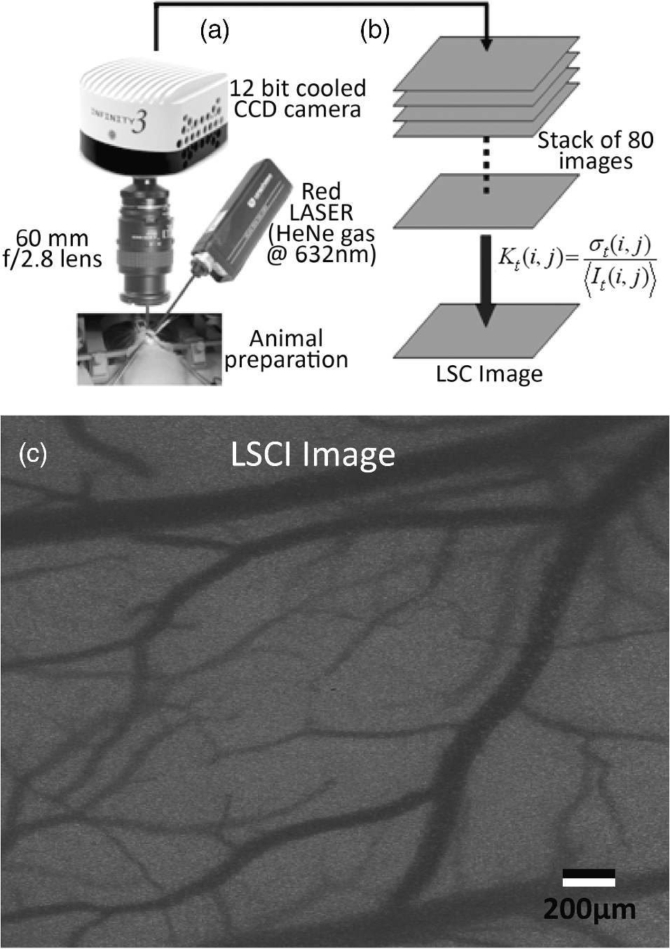 2.1.3.Longitudinal imaging over two weeksImaging was done at day 0 (baseline, just after tumor inoculation), day 3, day 7, day 10, and day 14 (biweekly for two weeks). On each of these days, animals were anesthetized, surgical clips were removed, and the thinned skull window was cleaned for imaging by flushing with saline and gently swabbing with a cotton-tipped applicator. In addition, on each imaging day, the skull needed to be minimally re-thinned to achieve the approximate optical clarity seen on day 0. Some of the larger blood vessels were used for gross registration of the FOV to the LSCI image obtained on day 0. Then imaging was done as described above to obtain a corresponding LSCI image for each animal on each imaging day. After the completion of imaging on each of the days, the skin was closed with surgical clips, and the animals were returned to the housing facility. After day 14, LSCI images obtained on each imaging day were manually registered to the LSCI image obtained on day 0, and the region of interest was cropped appropriately. It was difficult to achieve perfect registration or to use an automatic approach because of the physical displacement of vessels by the tumor growing inside the intracranial cavity. 2.1.4.Tumor confirmationHistology was done to confirm the presence and location of the tumor. At the end of our imaging on day 14, we sacrificed the animals using intracardiac perfusion with saline followed by 4% paraformaldehyde. Brains were harvested and sectioned, some in the coronal plane and some in the axial plane, both centered close to the tumor site. Following this, we performed a standard H&E stain to confirm the presence and location of the tumor. In addition, to confirm the precise location of the inoculated tumor, two tumor-bearing rats were imaged using MRI on days 10 and 14 in a 4.7 Tesla magnetic field scanner. Rats were anesthetized with halothane, immobilized in a plastic tube, intubated, and kept under anesthesia during MRI. Eight coronal and eight transverse sections were acquired. Each transverse slice had a FOV of and a thickness of 1 mm. The coronal sections had a FOV of . The pixel size in both sections was . 2.2.Data AnalysisThe LSCI images obtained from longitudinal imaging experiments were processed for extraction of MVD. MVD was estimated as the number of nodes in a unit area of the LSCI image. A node was either an endpoint of a blood vessel or an intersection point (where a parent vessel branches into two daughter vessels). In essence, we transformed the problem of counting the number of vessel segments in a region to counting the number of intersection points and endpoints of vessels, since the latter count is unique to a defined area. 2.2.1.Spatiotemporal study of MVDWe employed a custom written MATLAB (Mathworks, Massachusetts) program to count and calculate localized MVD values over the entire FOV. The program first displayed the obtained LSCI image, on which the user manually identified nodes, that is, intersection and end points of vessels. Figure 2(a) shows an example LSCI image with all nodes identified. The program proceeds to automatically calculate and represent the spatial distribution of MVD by counting the number of identified nodes within fixed or moving windows over the entire FOV. The manually identified nodes were counted and displayed using colored overlays. Counting of nodes was done within each square of a virtual overlaid grid, as shown in Fig. 2(b). We used a grid in which each square measured (). To obtain spatially continuous trends of MVD, as shown in Fig. 2(c), we also counted the number of nodes within a moving circular window around every pixel. If represents the complete set of identified nodes, the MVD at pixel location on the image was calculated as size (), where Fig. 2Estimation and display of MVD. (a) An example LSCI image of the rat’s cerebral vasculature, overlaid with a virtual grid for MVD estimation. Each square of the grid is . The white dots indicate vessel intersection points and endpoints that have been manually picked toward MVD estimation. (b) The MVD count in pseudo color in each square of the grid. MVD is calculated by counting the number of vessel endpoints and intersection points in each square and multiplying by four (so that MVD is expressed per ). (c) A continuous spatial map of MVD values calculated in a circular neighborhood around every pixel. The black dots in (c) correspond to the white dots in (a).  For each pixel, we counted the number of nodes in a circular area (radius ) around it to calculate the MVD at that pixel. Evaluating the MVD at every pixel in the image gave us a continuous MVD trend over the entire FOV. This information was color coded and overlaid on the LSCI images. 2.2.2.Statistical analysisWe performed a longitudinal study using LSCI in 10 tumor-bearing rats, six saline-injected rats, and 11 control rats. We tracked MVD values twice a week over two weeks of tumor growth. While the average survival of tumor-bearing rats was 17 days, imaging for two weeks was adequate. Beyond two weeks, the tumor size was significantly large inside the rat’s brain, a phase that is equivalent to the terminal phase in humans. Such advanced brain tumors are well beyond medication and/or surgical intervention, and their analogs were not imaged. MVD was estimated as described earlier, and statistical inferences were made. The number of rats in each group was unequal, since not all rats in each group met the inclusion criterion that LSCI image data be available on each of the five imaging sessions until day 14. This is attributable to premature death in some cases or a compromised thinned skull preparation. All available data meeting this criterion was reported and included in the statistical assessment. For the data to be included in the tumor group, it was necessary that the tumor was present in the appropriate region as seen in histological sections. A Mann Whitney test was performed on LSCI data obtained from the three groups and the five imaging sessions. 3.ResultsOur LSCI-based platform made it possible to monitor angiogenesis longitudinally. The degree of neovascularization that is typical in tumor environments was quantified in terms of MVD. On one hand, we studied the temporal changes in MVD by imaging the rodent on days 0, 3, 7, 10, and 14. On the other hand, the wide-field nature of LSCI also allowed us to study the spatial variation of MVD. 3.1.LSCI Can Visualize Remodeling of Brain Microvasculature in Longitudinal ExperimentsFigure 3(a) and 3(b) shows the LSCI images of rat brain microvasculature obtained on the day of tumor inoculation and 10 days after inoculation, respectively. They clearly demonstrate the ability of LSCI to visualize the changes in vascular architecture and the appearance of new vessels. The entire region of interest (ROI) has been divided into 15 squares with an area of to enable a spatial comparison of vascular remodeling. The number of vessel segments was counted manually in each square. For example, in square (2,3), which lies above the inoculation site, the vessel count increased from 17 on day 0 to 29 on day 10, suggesting robust neovascularization. From Fig. 3, one can also observe that the original vasculature remains intact, thus allowing us to register the two images for comparison, but the addition of new vasculature makes it extremely difficult for any automated registration schemes to achieve the same. Fig. 3LSCI images reveal long-term vascular remodeling. LSCI images of the rat brain region of interest obtained (a) on the day of tumor inoculation and (b) 10 days after inoculation. The two images have been registered manually, and the entire area has been broken down into a square grid labeled (1,1) to (3,5). 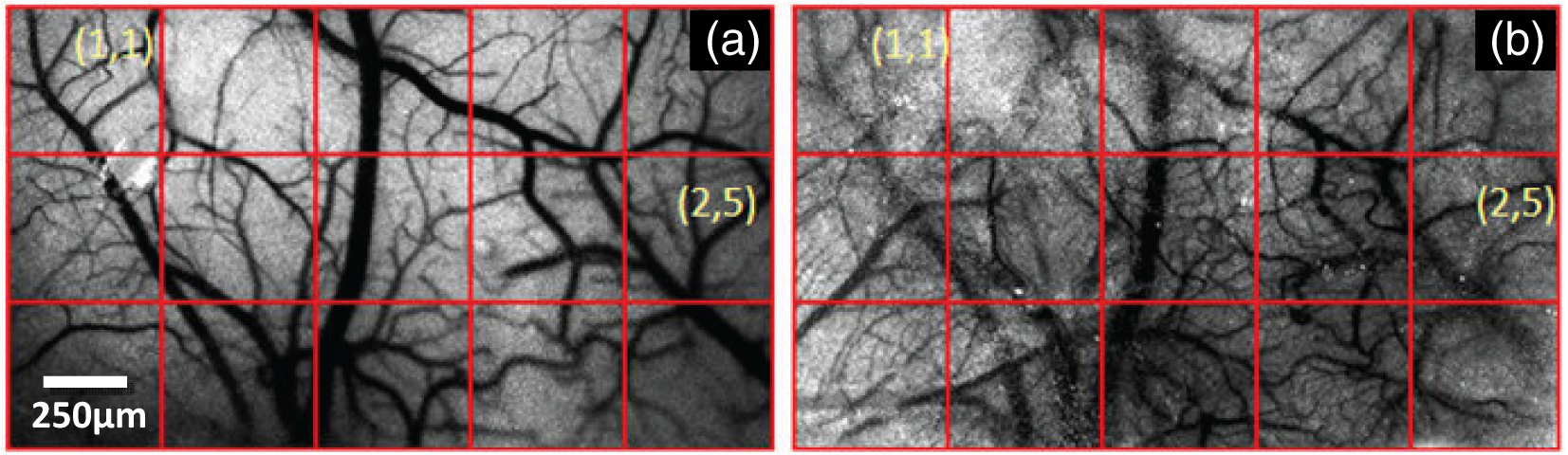 Histology was used to confirm the presence and location of the tumor post mortem. Figure 4 shows H&E stained axial sections of two rats along with day 14 LSCI images to provide the readers an estimate of the size and location of the inoculated tumors with respect to the imaged ROI. Data from the tumor group was used for statistical analysis only if the tumor was visible and appropriately located under the imaging window. In an odd occurrence, one of the supposed tumor-bearing rats did not show a tumor in the histological sections, which implied that the inoculated cells had not developed into a tumor. Such data was discarded. Ten rats showed intracranial tumors and constituted the tumor group. Fig. 4Confirming tumor location under imaging window using histology. H&E staining was used to confirm tumor location. (a) and (d) show the LSCI images acquired of the region of interest before sacrifice. (b) and (c) clearly show the tumor on day 14 in the axial section with the box indicating the location of the imaging window with respect to the whole brain and tumor. The presence of tumor under the imaging window was used as a criterion for inclusion of data in the tumor group.  3.2.Spatial Assessment of Microvessel Density over Tumor Growth CourseWe demonstrated the capability of LSCI to quantitatively assess the microvascular structure and morphology before and after tumor angiogenesis in terms of MVD. MVD was estimated by manually picking intersection and endpoints of vessels in each LSCI image. Counting the nodes produced intuitive color-coded MVD maps, as in Fig. 2, which were overlaid on the original LSCI images. This allowed us to compare the extent of neovascularization quantitatively in terms of increase in MVD over the baseline. Figure 5 shows a comparison of one control (unperturbed) rat brain and one tumor-bearing rat brain on days 0, 7, and 14. These continuous MVD maps show a rapid increase in MVD in the tumor-bearing animal, while the control shows only minor variation. All MVD maps are scaled similarly. The MVD map of the tumor-bearing animal clearly showed a hot spot with a high degree of vascularity, seen as a red patch in Fig. 5. The peak MVD at this hot spot was , in comparison to an average MVD of in the baseline image. The hot spot roughly correlated with the site of inoculation. However, since the tumor was fairly big on day 14, it remains to be seen how precisely the hot spot correlates with tumor location and size. Fig. 5Spatiotemporal comparison of MVD values in tumor-bearing and control rats. The images show continuous MVD maps overlaid on the cerebral vasculature of an animal from the unperturbed control group (left panel) and the tumor-bearing group (right panel) on days 0, 7, and 14 after baseline imaging and/or tumor injection. All images are scaled to the same color map (as indicated). The change in MVD over time in the control animal is small, whereas a steep increase in MVD is observed in the tumor-bearing animal.  3.3.Temporal MVD Trends in Tumor-Bearing Rats and ControlsMVD values were estimated across the FOV in all 27 rats (10 tumor-bearing, six saline-receiving controls, and 11 unperturbed controls) over the five imaging sessions. Figure 6 shows the trend of mean MVD values over the entire ROI through the two-week course of tumor growth. The tumor group shows a sharp increase in MVD relative to day 0, while both the control groups witnessed an increasing-decreasing trend in MVD. The inset table reports the groupwise statistical significance ( values) on each imaging day calculated using the Mann Whitney test. There is a statistically significant difference () between the MVD values of the tumor group and both the control groups on days 3 through 14. However, there is weaker evidence of the two control groups being different () on days 3 through 10. On day 14, there is strong evidence that both the saline-receiving group and the unperturbed group belong to the same distribution (). On day 14, the tumor group exhibited relative MVD values of , which was significantly higher than the aggregated mean of both control groups of (). On day 14, absolute MVD values were also significantly higher in the tumor group () than in the unperturbed control group (, ) or the saline-receiving control group (, ). Fig. 6Longitudinal variation of MVD over the course of tumor growth. Three groups—tumor (), saline controls (), and unperturbed controls ()—were monitored using LSCI over two weeks since the day of inoculation (day 0). The plot shows means and standard error bars of the MVD averaged over the ROI and normalized to its corresponding baseline MVD value on day 0. The inset table shows results ( value) of a Mann Whitney U test performed to compare the three experimental groups pairwise. The asterisk indicates statistical significance () between groups. The dagger indicates that the day 14 MVD of the saline and unperturbed groups belong to the same distribution.  4.DiscussionThe goal of this paper was to assess the suitability of LSCI for longitudinal imaging of the brain tumor microenvironment through a thinned skull. Toward this, we demonstrated and characterized a novel method of estimating and visualizing microvessel density to assess quantitatively the long-term vascular remodeling that accompanies brain tumor progression. MVD was estimated in terms of the number of intersection points and endpoints of blood vessels per unit area. It must be noted that it was necessary to modify our cranial window by thinning the skull marginally with a drill prior to each imaging session to retain the optical clarity. Repeated thinning of the skull often results in skull opacity after the fifth thinning session. Thus, if the study requires frequent or longer-term monitoring of the ROI, we recommend implanting a glass window into the skull.36 However, in such a preparation, unlike the thinned skull preparation, the brain is not in its native state, which may affect the course of tumor growth and vascular response. 4.1.LSCI Can Visualize Remodeling of Brain Microvasculature in Longitudinal ExperimentsLSCI has conventionally been used as a blood flow imaging technique, and hence LSCI users have used a spatial processing scheme that involves calculation of speckle contrast in the spatial domain; that is, is calculated in a sliding window (typically ) across a single acquired raw laser speckle image. This scheme compromises on the spatial resolution and cannot discern the extent of new vessel formation. For assessment of microvascular changes that characterize tumor environments, a high-resolution temporal scheme needed to be utilized.3,35 Figure 7(a)–7(d) shows a comparison of the difference in resolution as seen with the spatial and temporal processing schemes of the same raw LSCI data obtained on day 0 and day 3 in one of our experimental rats. We observed that the improvement in resolution enabled the identification of tumor-associated neovasculature, which comprises of microvessels less than 15 microns in diameter. We analyzed the enhancement provided by the temporal scheme in estimating MVD by comparing MVD values achievable using the temporal and spatial schemes in each square of a square grid overlaid on the ROI. This was done in 15 images (three rat brains over five imaging sessions), and the results are shown in Fig. 7(e). The median and quartiles over 15 images of the maximum density of nodes in each image were calculated and compared for the spatial and temporal schemes. The temporal scheme was shown to perform significantly better for imaging microvessels, and it was able to discern tumor-associated vascular remodeling. We have previously demonstrated the utility of LSCI for monitoring angiogenesis that accompanies wound healing in a mouse ear model,37 and now, we demonstrate its utility to image vascular remodeling in the brain and skull. It must also be noted that the temporal scheme is sensitive to motion artifact, such as brain pulsations that could become more significant in bigger animals. Miao et al. have previously described a scheme of registering the raw frames to one another before speckle contrast is calculated, to address such motion artifact.38 Fig. 7Demonstration of the utility of LSCI with a temporal processing scheme to identify tumor-associated neovasculature. Baseline LSCI images of rat cerebral vasculature were taken using (a) traditional/spatial processing and (b) temporal processing. Equivalent (c) spatially and (d) temporally processed LSCI images were taken after the tumor was grown for several days. Note the improved resolution of (b) versus (a) and (d) versus (c). Also note the neovascularization evident in comparing (d) with (b). (e) A statistical comparison of the utility of the two schemes for microvessel identification. The median and quartiles are plotted for MVD values measured (). Images have been scaled uniformly and linearly to improve print reproduction.  4.2.Spatial Assessment of Microvessel Density over Tumor Growth CourseThe LSCI modality, in conjunction with the MVD estimation and display techniques, enables serial assessment microvascular remodeling in the same rat over several days. This makes it possible to normalize the MVD values to the baseline MVD and study the temporal variation of MVD in each rat. We observed that there was significant variation in baseline MVD values of each rat of ; that is, a standard deviation as high as 28% of the mean. This finding suggests that MVD trends need to be monitored independently for every rat, rather than being averaged over the entire cohort. Hence, LSCI-based monitoring provides an inherent advantage over classical terminal techniques of monitoring angiogenesis such as histology and immunohistochemistry, where it is impossible to monitor trends individually for every rat. The large FOV of LSCI allows for monitoring of microvessels overlying the entire spatial spread of the tumor mass. As can be seen from Fig. 4, the size of the tumor on day 14 is comparable to the size of the imaging window. Spatial assessment of MVD showed regions of increased MVD or hot spots (see the red region in Fig. 5). While these hot spots appear in regions overlying the tumor, the precise correlation between the associated MVD values and the tumor location and size remains to be investigated. At the same time, it must be appreciated that LSCI is a surface imaging modality and provides a 2D rendition of the ROI overlying the tumor. The depth of imaging is limited by the penetration of red (632-nm) laser in brain tissue. While use of a longer wavelength in the near infrared or infrared regime can improve the depth range, the same would compromise the in-plane spatial resolution, since the size of laser speckles is proportional to the wavelength.39 Alternatively, LSCI could be complemented with other optical imaging technologies such as optical frequency domain imaging, which can resolve the tumor microenvironment depth-wise.21 In our experiments, the glioma cells were introduced as superficially as possible into the intracranial cavity, roughly 2 mm below the surface of the thinned skull, so that vascular changes extend to the surface as the tumor grows. For confirmation, MRI was done on two randomly chosen tumor-bearing rats on days 10 and 14. As shown in Fig. 8, the center of the tumor was confirmed from these images to be about 3 to 3.5 mm from the midline and about 2 to 2.5 mm from the surface of the thinned skull preparation. However, the tumor was also estimated to reach up to approximately 1.5 mm from the surface, as a hint of the tumor is seen in the topmost transverse section. The location of the tumor co-registered well with the thinned skull monitoring window. Fig. 8The site of tumor inoculation. (a) Coronal section stained with H&E. (b) Coronal T2 weighted MRI section. These images confirm that the glioma cells were inoculated at a depth of approximately 2 mm from the surface. (c) Transverse T2 weighted MRI sections confirm the tumor mass extends to within 1.5 mm from the surface (section D-D). All images shown were obtained on day 14. 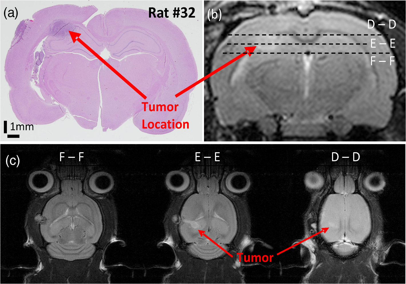 Neovascularization is often measured by estimating vascular length or equivalently functional vascular density40 (FVD). Spatial MVD maps were found to be significantly correlated (correlation coefficient , ) to spatial FVD maps across all five imaging sessions in both tumor () and unperturbed control () rat brains. However, since our goal was assessing tumor environments, it was important to have a parameter such as MVD that was sensitive to short branching microvessels as are associated with neoplasia, rather than long nonbranching segments. 4.3.Temporal MVD Trends in Tumor-Bearing Rats and ControlsWhen imaging the rodent glioma model through a thinned skull, the brain encountered three types of insults. First, the thinning of the skull triggered a wound healing response, which is accompanied by neovascularization. Second, the act of injecting a liquid mass (tumor or saline) into the brain using a Hamilton syringe created an insult that is expected to trigger an immune response of its own. Finally, our targeted insult consisted of introducing glioma cells into the brain, since the goal of the study was the monitor the effect of those cells. Our three groups of rodents—the unperturbed controls, the saline-receiving controls, and the tumor-receiving experimental group—helped us decouple the specific effects of each insult as pertains to vascular remodeling. After a large amount of skull thinning on day 0, there was expectedly an immediate thermoregulatory and healing response that increased blood flow to the thinned skull within the FOV through redundancies, thereby causing the measured MVD values in the ROI to appear elevated in all three groups. On days 3 to 14, skulls were re-thinned only marginally. Hence, on these days, this marginal secondary insult did not produce as much of an increase in measured MVD as on day 0. As shown in Fig. 6, days 3 and 7 were marked with progressively increasing MVD, a result of long-term neovascularization that accompanies the healing skull. The difference in the relative MVDs among the three groups on days 3 and 7 are attributed to the difference in the injected mass. MVD values in the tumor group were significantly different from the controls, while the difference between the two control groups was only weakly significant (), possibly due to a residual effect caused by the second type of insult. Day 10 witnessed decreasing neovascularization due to the first two types of insults, but the tumor group showed consistently high MVD values. Finally, on day 14, the two control groups showed the same level of vascularization (), suggesting that the vascular remodeling effect of the first two types of insults had nearly completed, and the MVD values had returned to a true baseline, which was different from day 0 MVD values, since the latter represented the effect of significant bone thinning. On day 14, the MVD values in the tumor group were significantly higher than the values in both control groups, suggesting an exclusive effect of tumor growth and vascular recruitment. Figure 5 shows a representative spatial distribution of this confounded multi-insult vascular remodeling response over the two-week period. The intermittent increase in MVD in the unperturbed controls on day 7 can be attributed to wound healing, while the progressive increase in MVD in the tumor-bearing animal can be attributed to a combination of wound healing and tumor on day 7 but predominantly tumor on day 14. Thus, as this paper demonstrates, skull thinning triggers a wound healing response that needs to be accounted for when conducting longitudinal studies. Other disadvantages of the thinned skull preparation include a limited ability to visualize only the surface of the brain and poor tissue depth penetration due to the surface imaging nature of LSCI. In addition, there is no objective way of ensuring the same skull thickness during different imaging sessions, which can result in variable image quality. However, a compelling reason to employ the thinned skull preparation is that it preserves the integrity of the brain microeonvironment, allowing the disease model to mimic naturally occurring physiological conditions. In the case of brain tumors, such conditions include progressively rising intracranial pressure as the tumor grows, as well as the chemical and immunological balance associated with an uncompromised brain. 4.4.Potential ApplicationsThe ability of LSCI of imaging tumor-associated vascular remodeling lends itself to various laboratory and clinical applications. This method could find application in anti-angiogenic drug studies, whereby the efficacy and spatiotemporal effects of the drug on vasculature could be studied. Through appropriate experimental design, it becomes possible to study not only the effect of anti-angiogenic drugs on tumors, but also their side effects on wound healing. Drug doses can be titrated based on the temporal rate of decay of MVD values in presence of the drug or the spatial outreach of vascular disruption over the wide FOV. In addition to high-resolution structural imaging, LSCI can image the blood flow through microvessels, thereby adding another dimension to angiogenesis research. Drug delivery to proximal and distal sites, especially in the context of new concepts like vascular normalization,41,42 can be probed using the same platform. In the rodent glioma model with an initial injection of 100,000 9L cells, the size of the tumor on day 14 is analogous to a clinical situation in humans, when surgical intervention is likely. Tumor resection is a delicate balance between removing as much tumor as possible and leaving behind as much healthy tissue as possible. In such a critical surgery, LSCI has the potential to assist the neurosurgeon with informative MVD maps of the FOV. Unlike complicated equipment like intraoperative MRI scanners,43 the LSCI equipment is simple and can be easily integrated into the operating room. On day 14, absolute MVD values were also significantly higher in the tumor group than in the unperturbed control group () and the saline-receiving control group (). This result, in conjunction with the presence of elevated MVD hot spots on the spatial MVD map, provides preliminary evidence that MVD could be used to discriminate tumors intraoperatively. Further, it is possible to automate the estimation of MVD using advanced computational vessel segmentation approaches44 to facilitate its objective use in the laboratory or clinic. Our study used manual identification of vessel intersection and endpoints as the gold standard to obviate any error associated with automatic approaches. White, George, and Choi have reported a method of segmenting vessels from LSCI images and subsequently skeletonizing the vessels to their respective single-pixel-thick centerlines to estimate vessel length.45 Vessel intersection points and endpoints could be identified automatically as pixels on these vessel skeletons that have three neighbors and one neighbor, respectively, forming the basis for MVD calculation. However, the accuracy of such automated algorithms remains to be determined. 5.ConclusionLSCI is well suited to image the microvascular remodeling that is typical in tumor environments. Intrinsic advantages of LSCI include its wide-field and high-resolution images and its lack of dependence for any external contrast agent, allowing for serial imaging of rat brains over multiple sessions. We added a quantitative capability to the imaging modality by extracting, counting, and displaying MVD over the entire FOV, setting up an imaging platform for angiogenesis research. LSCI was able to monitor the progressive increase in MVD through the growth course of the brain tumor. LSCI was also able to discriminate the tumor-associated high MVD values from low control MVD values on the 14th day after inoculation, suggesting, in a preliminary manner, that LSCI-based imaging systems may assist in tumor resection for neurosurgeons in the operating room by providing MVD maps of the surgical FOV. AcknowledgmentsThis work was supported jointly by National Institute of Aging award number R01AG029681 and Department of Health and Human Services award number 1R43CA139983-01. The authors would like to thank Dr. Violette Recinos for help with tumor inoculation and initial model development. Also, we acknowledge the contributions of Kartikeya Murari, Nan Li, Saurabh Kalra, and Dr. David Sherman on various optical imaging-related aspects of this work. ReferencesC. Ayataet al.,
“Laser speckle flowmetry for the study of cerebrovascular physiology in normal and ischemic mouse cortex,”
J. Cereb. Blood Flow Metab., 24
(7), 744
–755
(2004). http://dx.doi.org/10.1097/01.WCB.0000122745.72175.D5 JCBMDN 0271-678X Google Scholar
J. D. BriersS. Webster,
“Laser speckle contrast analysis (LASCA): a nonscanning, full-field technique for monitoring capillary blood flow,”
J. Biomed. Opt., 1
(2), 174
–179
(1996). http://dx.doi.org/10.1117/12.231359 JBOPFO 1083-3668 Google Scholar
K. Murariet al.,
“Contrast-enhanced imaging of cerebral vasculature with laser speckle,”
App. Opt., 46
(22), 5340
–5346
(2007). http://dx.doi.org/10.1364/AO.46.005340 APOPAI 0003-6935 Google Scholar
N. Liet al.,
“High spatiotemporal resolution imaging of the neurovascular response to electrical stimulation of rat peripheral trigeminal nerve as revealed by in vivo temporal laser speckle contrast,”
J. Neurosci. Methods, 176
(2), 230
–236
(2009). http://dx.doi.org/10.1016/j.jneumeth.2008.07.013 JNMEDT 0165-0270 Google Scholar
J. Folkman,
“Tumor angiogenesis: therapeutic implications,”
N. Engl. J. Med., 285
(21), 1182
–1186
(1971). http://dx.doi.org/10.1056/NEJM197111182852108 NEJMBH Google Scholar
E. P. Siposet al.,
“Inhibition of tumor angiogenesis,”
Ann. New York Acad. Sci., 732 263
–272
(1994). http://dx.doi.org/10.1111/nyas.1994.732.issue-1 ANYAA9 0077-8923 Google Scholar
J. E. Wolffet al.,
“Dexamethasone reduces vascular density and plasminogen activator activity in 9L rat brain tumors,”
Brain Res., 604
(1–2), 79
–85
(1993). http://dx.doi.org/10.1016/0006-8993(93)90354-P BRREAP 1385-299X Google Scholar
W. Figget al., Angiogenesis, 321
–332 Springer, United States
(2008). Google Scholar
P. R. ValeJ. M. IsnerK. Rosenfield,
“Therapeutic angiogenesis in critical limb and myocardial ischemia,”
J. Interv. Cardiol., 14
(5), 511
–528
(2001). http://dx.doi.org/10.1111/j.1540-8183.2001.tb00367.x JICAF2 Google Scholar
I. Tropreset al.,
“In vivo assessment of tumoral angiogenesis,”
Magn. Reson. Med., 51
(3), 533
–541
(2004). http://dx.doi.org/10.1002/(ISSN)1522-2594 MRMEEN 0740-3194 Google Scholar
T. G. PurdieE. HendersonT. Y. Lee,
“Functional CT imaging of angiogenesis in rabbit VX2 soft-tissue tumour,”
Phys. Med. Biol., 46
(12), 3161
–3175
(2001). http://dx.doi.org/10.1088/0031-9155/46/12/307 PHMBA7 0031-9155 Google Scholar
G. NiuX. Chen,
“PET imaging of angiogenesis,”
PET Clin., 4
(1), 17
–38
(2009). http://dx.doi.org/10.1016/j.cpet.2009.04.011 Google Scholar
B. Turkbeyet al.,
“Imaging of tumor angiogenesis: functional or targeted?,”
Am. J. Roentgenol., 193
(2), 304
–313
(2009). http://dx.doi.org/10.2214/AJR.09.2869 AJROAM 0092-5381 Google Scholar
T. Oritaet al.,
“The microvascular architecture of human malignant glioma. A scanning electron microscopic study of a vascular cast,”
Acta. Neuropathol. (Berl.), 76
(3), 270
–274
(1988). http://dx.doi.org/10.1007/BF00687774 ANPTAL 1432-0533 Google Scholar
P. VajkoczyM. D. Menger,
“Vascular microenvironment in gliomas,”
J. Neuro-Oncol., 50
(1–2), 99
–108
(2000). http://dx.doi.org/10.1023/A:1006474832189 Google Scholar
T. Motoikeet al.,
“Universal GFP reporter for the study of vascular development,”
Genesis, 28
(2), 75
–81
(2000). http://dx.doi.org/10.1002/(ISSN)1526-968X 1526-954X Google Scholar
N. W. Galeet al.,
“Ephrin-B2 selectively marks arterial vessels and neovascularization sites in the adult, with expression in both endothelial and smooth-muscle cells,”
Dev. Biol., 230
(2), 151
–160
(2001). http://dx.doi.org/10.1006/dbio.2000.0112 DEBIAO 0012-1606 Google Scholar
R. F. GarianoT. W. Gardner,
“Retinal angiogenesis in development and disease,”
Nature, 438
(7070), 960
–966
(2004). http://dx.doi.org/10.1038/nature04482 NATUAS 0028-0836 Google Scholar
C. C. Reyes-Aldasoroet al.,
“Estimation of apparent tumor vascular permeability from multiphoton fluorescence microscopic images of P22 rat sarcomas in vivo,”
Microcirculation, 15
(1), 65
–79
(2008). http://dx.doi.org/10.1080/10739680701436350 Google Scholar
S. G. AdieS. A. Boppart, Optical Imaging of Cancer, 209
–250 Springer, New York
(2009). Google Scholar
B. J. Vakocet al.,
“Three-dimensional microscopy of the tumor microenvironment in vivo using optical frequency domain imaging,”
Nat. Med., 15
(10), 1219
–1223
(2009). http://dx.doi.org/10.1038/nm.1971 1078-8956 Google Scholar
H. J. Böhringeret al.,
“Time-domain and spectral-domain optical coherence tomography in the analysis of brain tumor tissue,”
Lasers Surg. Med., 38
(6), 588
–597
(2006). http://dx.doi.org/10.1002/(ISSN)1096-9101 LSMEDI 0196-8092 Google Scholar
S. HuL. V. Wang,
“Photoacoustic imaging and characterization of the microvasculature,”
J. Biomed. Opt., 15
(1), 011101
(2010). http://dx.doi.org/10.1117/1.3281673 JBOPFO 1083-3668 Google Scholar
R. Steinmeieret al.,
“Laser Doppler flowmetry mapping of cerebrocortical microflow: characteristics and limitations,”
NeuroImage, 15
(1), 107
–119
(2002). http://dx.doi.org/10.1006/nimg.2001.0943 NEIMEF 1053-8119 Google Scholar
A. Limbourget al.,
“Evaluation of postnatal arteriogenesis and angiogenesis in a mouse model of hind-limb ischemia,”
Nat. Protocols, 4
(12), 1737
–1748
(2009). http://dx.doi.org/10.1038/nprot.2009.185 1754-2189 Google Scholar
A. RegeN. V. ThakorA. P. Pathak,
“Optical imaging of blood vessel morphology and function,”
Curr. Angiogenesis, 1
(3), 243
–260
(2012). http://dx.doi.org/10.2174/2211552811201030243 2211-5528. Google Scholar
E. Kimet al.,
“Multiscale imaging and computational modeling of blood flow in the tumor vasculature,”
Ann. Biomed. Eng., 40
(11), 2425
–2441
(2012). http://dx.doi.org/10.1007/s10439-012-0585-5 ABMECF 0090-6964 Google Scholar
A. Mooreet al.,
“Novel gliosarcoma cell line expressing green fluorescent protein: a model for quantitative assessment of angiogenesis,”
Microvasc. Res., 56
(3), 145
–153
(1998). http://dx.doi.org/10.1006/mvre.1998.2102 MIVRA6 0026-2862 Google Scholar
M. A. Badruddojaet al.,
“Antiangiogenic effects of dexamethasone in 9L gliosarcoma assessed by MRI cerebral blood volume maps,”
Neuro-Oncology, 5
(4), 235
–243
(2003). http://dx.doi.org/10.1215/S1152851703000073 JNODD2 0167-594X Google Scholar
M. Guoet al.,
“9L gliosarcoma cell proliferation and tumor growth in rats are suppressed by N-hydroxy-N’-(4-butyl-2-methylphenol) formamidine (HET0016), a selective inhibitor of CYP4A,”
J. Pharmacol. Exp. Ther., 317
(1), 97
–108
(2006). http://dx.doi.org/10.1124/jpet.105.097782 JPETAB 0022-3565 Google Scholar
B. A. Moffatet al.,
“Inhibition of vascular endothelial growth factor (VEGF)-A causes a paradoxical increase in tumor blood flow and up-regulation of VEGF-D,”
Clin. Cancer Res., 12
(5), 1525
–1532
(2006). http://dx.doi.org/10.1158/1078-0432.CCR-05-1408 1078-0432 Google Scholar
D. YoshidaY. IkedaS. Nakazawa,
“Copper chelation inhibits tumor angiogenesis in the experimental 9L gliosarcoma model,”
Neurosurgery, 37
(2), 287
–293
(1995). http://dx.doi.org/10.1227/00006123-199508000-00014 JONSAC 0022-3085 Google Scholar
J. Duda-SzymanskaW. Papierz,
“Morphological analysis of vascular density in ependymomas,”
Folia Neuropathol., 45
(3), 115
–119
(2007). 1641-4640 Google Scholar
D. Coolet al.,
“Tissue-based affine registration of brain images to form a vascular density atlas,”
in 6th Intl. Conf. Med. Imag. Comp. Comput. Asst. Intervention (MICCAI),
9
–15
(2003). Google Scholar
H. Chenget al.,
“Modified laser speckle imaging method with improved spatial resolution,”
J. Biomed. Opt., 8
(3), 559
–564
(2003). http://dx.doi.org/10.1117/1.1578089 JBOPFO 1083-3668 Google Scholar
D. Abookasiset al.,
“Imaging cortical absorption, scattering, and hemodynamic response during ischemic stroke using spatially modulated near-infrared illumination,”
J. Biomed. Opt., 14
(2), 024033
(2009). http://dx.doi.org/10.1117/1.3116709 JBOPFO 1083-3668 Google Scholar
A. Regeet al.,
“Multi exposure laser speckle contrast imaging of the angiogenic microenvironment,”
J. Biomed. Opt., 16
(5), 056006
(2011). http://dx.doi.org/10.1117/1.3582334 JBOPFO 1083-3668 Google Scholar
P. Miaoet al.,
“High resolution cerebral blood flow imaging by registered laser speckle contrast analysis,”
IEEE Trans. Biomed. Eng., 57
(5), 1152
–1157
(2010). http://dx.doi.org/10.1109/TBME.2009.2037434 IEBEAX 0018-9294 Google Scholar
S. J. KirkpatrickD. D. DuncanE. M. Wells-Gray,
“Detrimental effects of speckle-pixel size matching in laser speckle contrast imaging,”
Opt. Lett., 33
(24), 2886
–2888
(2008). http://dx.doi.org/10.1364/OL.33.002886 OPLEDP 0146-9592 Google Scholar
T. A. Readet al.,
“Intravital microscopy reveals novel antivascular and antitumor effects of endostatin delivered locally by alginate-encapsulated cells,”
Cancer Res., 61
(18), 6830
–6837
(2001). CNREA8 0008-5472 Google Scholar
D. A. I. FukumuraR. K. Jain,
“Imaging angiogenesis and the microenvironment,”
APMIS, 116
(7–8), 695
–715
(2008). http://dx.doi.org/10.1111/apm.2008.116.issue-7-8 APMSEL 0903-4641 Google Scholar
R. K. Jain,
“Normalization of tumor vasculature: an emerging concept in antiangiogenic therapy,”
Science, 307
(5706), 58
–62
(2005). http://dx.doi.org/10.1126/science.1104819 SCIEAS 0036-8075 Google Scholar
W. Hallet al.,
“3-Tesla intraoperative MR imaging for neurosurgery,”
J. Neuro-Oncol., 77
(3), 297
–303
(2006). http://dx.doi.org/10.1007/s11060-005-9046-4 JNODD2 0167-594X Google Scholar
C. KirbasF. K. H. Quek,
“Vessel extraction techniques and algorithms: a survey,”
in Proc. IEEE Sym. Bioinform. Bioengr.,
238
–245
(2003). Google Scholar
S. M. WhiteS. C. GeorgeB. Choi,
“Automated computation of functional vascular density using laser speckle imaging in a rodent window chamber model,”
Microvasc. Res., 82
(1), 92
–95
(2011). http://dx.doi.org/10.1016/j.mvr.2011.03.006 MIVRA6 0026-2862 Google Scholar
|


