Quantitative evaluation of skeletal muscle defects in second harmonic generation images

Wenhua Liu; Evelyn Ralston; Nina Raben

doi:10.1117/1.JBO.18.2.026005

1 February 2013 Quantitative evaluation of skeletal muscle defects in second harmonic generation images

Wenhua Liu, Evelyn Ralston, Nina Raben

Author Affiliations +

Journal of Biomedical Optics, Vol. 18, Issue 2, 026005 (February 2013). https://doi.org/10.1117/1.JBO.18.2.026005

Abstract

Skeletal muscle pathologies cause irregularities in the normally periodic organization of the myofibrils. Objective grading of muscle morphology is necessary to assess muscle health, compare biopsies, and evaluate treatments and the evolution of disease. To facilitate such quantitation, we have developed a fast, sensitive, automatic imaging analysis software. It detects major and minor morphological changes by combining texture features and Fourier transform (FT) techniques. We apply this tool to second harmonic generation (SHG) images of muscle fibers which visualize the repeating myosin bands. Texture features are then calculated by using a Haralick gray-level cooccurrence matrix in MATLAB. Two scores are retrieved from the texture correlation plot by using FT and curve-fitting methods. The sensitivity of the technique was tested on SHG images of human adult and infant muscle biopsies and of mouse muscle samples. The scores are strongly correlated to muscle fiber condition. We named the software MARS (muscle assessment and rating scores). It is executed automatically and is highly sensitive even to subtle defects. We propose MARS as a powerful and unbiased tool to assess muscle health.

1. Introduction

Skeletal muscle fibers and cardiac myocytes have a regular, periodic organization, which is not only structural but also functional.¹^–³ The repeating units, made largely of actin and myosin filaments, are called sarcomeres and are the structural basis for producing the force responsible for contractile function.⁴^–⁶ In a healthy muscle, sarcomeres, visualized in electron or light microscopy, appear as striations that are rarely interrupted and are in register between several neighboring fibers.⁷ Myopathies, such as Duchenne muscular dystrophy,⁸^,⁹ and metabolic disorders with muscle pathologies, such as Pompe disease,⁷^,¹⁰^,¹¹ affect the periodicity and the regularity of the sarcomeres, either by partial removal of contractile proteins or by inclusion of nonsarcomeric structures. Because progressive muscle weakness is the ultimate cause of death in such diseases, the ability to assess muscle condition quantitatively is highly desirable.

There are different ways to visualize sarcomeric organization. Electron microscopy produces very high-resolution views but of very small sample areas; preparation is lengthy.¹²^,¹³ Immunofluorescence, for example with anti-myosin or anti– $α$ -actinin antibodies, can be used but necessitates manual teasing to prepare single fibers that are separated from neighboring fibers, or the sectioning of muscle which again limits the sampling.¹³^,¹⁴ Two-photon microscopy provides an alternative technique, second harmonic generation imaging (SHG). SHG is a nonlinear optical effect created when a powerful pulsed laser passes through a highly polarized, non–centro-symmetric material.¹⁵^,¹⁶ The best SHG emitters are collagen and myosin. SHG microscopy can therefore be used to visualize the muscle sarcomere structure and has been used to visualize defects in mouse and human Pompe disease muscles without need for exogenous fluorophores and with minimum sample preparation.⁷^,¹⁷ An SHG endoscope even allows visualization of muscle sarcomeres in alert, unanesthetized animals and humans.¹⁸

A tool for the quantitative analysis of such images, sensitive to any kind of muscle defect, would be particularly useful for assessing long-term changes in patient biopsies or animal models, understanding disease evolution, assessing therapy, or testing new treatments. Plotnikov et al. proposed an imaging tool to evaluate muscle condition based on the notion that the spacing and angle of the sarcomeres can distinguish healthy from sick muscle.¹⁹ Their method is based on the calculation of pixel intensity and on comparisons with the neighboring pixels. Although this method works well for muscles with limited defects, it is not meant to analyze muscle fibers in which many or even most of the sarcomeres break down, such as in infants with Pompe disease.¹⁹

Friedrich et al.¹¹ and Garbe et al.²⁰ introduced another automatic tool by using the boundary tensor to detect verniers, which are local misalignments of sarcomere pattern. However, this method is limited to a particular defect of muscle structure. In Pompe disease, for example, there are several types of defects that could not be quantitated by this technique.

We have developed a novel imaging processing tool for detecting and quantifying muscle defects from SHG images. This software is based on texture analysis²¹^,²² and rates muscle condition by combining several mathematical and statistical tools. We have named it muscle assessment and rating scores (MARS). In this article we assess its potential for monitoring muscle disease by applying it to human and mouse samples.

As standards of reference we used muscle fibers from healthy human adults and from mice. As disease samples we examined biopsies of infants with Pompe disease, some of which we have imaged previously.⁷ Pompe disease is a lysosomal storage disorder resulting from the total or partial lack of the enzyme acid– $α$ -glucosidase.²³^–²⁵ The disease manifests itself as a cardiac and skeletal myopathy characterized by the presence in muscle fibers of enlarged, glycogen-filled lysosomes and of massive accumulations of autophagic debris. There are two major forms of the disease, infantile and late-onset. Before the development of the enzyme replacement therapy (ERT) infants died of heart failure within one to two years. ERT works well on cardiac muscle and has extended the lifespan of infants with Pompe disease. However, the treatment only partially alleviates the skeletal muscle problems, and not all patients respond similarly. It is therefore important to continue and try to better understand the disease. In particular it would be useful to find out how much clinical symptoms correlate with muscle defects observed by cell biological techniques. A technique for quantitating muscle defects is necessary to achieve this goal.

Our results show strong correlations between the rating scores and the Pompe muscle condition. We find that MARS is highly sensitive to subtle pattern disruptions and can be used to detect gradual microarchitecture changes during chronic disease development or during recovery after muscle treatments. We also demonstrate that MARS results are robust when imaging parameters (brightness and noise) vary. Once the image area to analyze has been selected, MARS functions automatically. Therefore MARS could give fast and unbiased assessment for evaluating muscle conditions regardless of the type of muscle defects and could be extended, with little additional work, to the analysis of other tissues.

2. Materials and Methods

2.1.

Muscle Biopsies: Origin and Preparation

Muscle fibers from a healthy, fasting, Caucasian male (age 33 years) were donated by Thorkil Ploug, MD (Department of Biomedical Sciences, University of Copenhagen, Denmark). The muscle fibers were from a biopsy obtained from m. vastus lateralis after local anesthesia of the skin and muscle fascia (Lidocain $5 mg / ml$ ; SAD, Copenhagen, Denmark) using the Bergström technique with suction.²⁶ Part of the biopsy was pinned down at resting length in a Petri dish coated with Sylgard 184 (Dow Corning Corporation, Midland, Michigan), incubated with Krebs-Henseleit bicarbonate buffer containing procaine hydrochloride ( $1 g / l$ ) for 3 min followed by 2% freshly depolymerized paraformaldehyde and 0.15% picric acid in 0.1 M phosphate buffer for 5 h. The fixed fibers were then stored in 50% glycerol in PBS at $- 20 ° C$ . The study adhered to the Helsinki II declaration, was approved by the Ethical Committee of Copenhagen (H-4-2009-089) and registered at the Danish Data Protection Agency (2009-41-3682).

Muscle biopsies from Pompe patients described in Refs. 24 and 27, and from a child with a mitochondrial disease unrelated to Pompe, were used in this research. The study was approved by local institutional review boards at all sites. Mouse muscle fibers were from the tibialis anterior (TA) muscle of wild-type mice. After euthanasia by ${CO}_{2}$ inhalation (following NIH guidelines), the whole leg was fixed by immersion into 4% parformaldehyde in 0.1 M phosphate buffer. Human muscle biopsies were also fixed with 4% parformaldehyde in 0.1 M phosphate buffer as soon as possible after collection. All muscle samples were kept at $- 20 ° C$ in 50% glycerol in PBS until used. Bundles of $\sim 5$ to 100 fibers were mounted on glass slides in 50% glycerol in chambers made with one or two self-adhesive spacers and sealed with a no. 1.5 cover glass.

2.2.

SHG Microscopy

All images were collected on a Leica SP5 NLO confocal microscope with a 3W Mai Tai HP Ti:Sapphire laser (Newport/Spectra-Physics, Irvine, California). The excitation wavelength was 870 nm and a $40 \times 1.25$ NA oil immersion objective was used. The forward SHG signal was collected in the transmitted light detector after a $435 / 20$ band-pass and a 680 short-pass filter (Chroma Technology, Bellows Falls, Vermont). Images were acquired with Leica LASAF 2.3.1 software.

2.3.

Imaging Processing

A flowchart of our analysis procedure is shown in Fig. 1. All the procedures are performed in MATLAB 7.11 (MathWorks, Natick, Massachusetts). The images’ brightness and contrast are adjusted by histogram equalization to standardize the input to the program. Each image’s average sarcomeric separation (SS) and orientation relative to the muscle fiber axis are detected automatically by analyzing the location and orientation of the peaks corresponding the sarcomeres in the Fourier spectrum of the original image. For fibers in extremely bad condition, manually measuring the SS and orientation is also necessary. Because these two parameters are very important for the final scores, the values will also be verified at later steps. The program then generates a set of gray-level, cooccurrence matrices (GLCM), a quantitative measure for the texture features proposed by Haralick et al.²¹ The dimensions of the matrices are the number of gray levels in the images (i.e., 256 for 8-bit images). To avoid artefacts due to very small intensity fluctuations and to accelerate calculations we bin the gray levels into eight values. For each pixel of the image we then compare its gray level $i$ to the gray level $j$ of a pixel separated in the fiber axis direction by a distance $d$ (the offset). This is repeated for each value of $d$ from $d = 1$ to $d = 4 \times S S$ (in pixels). One matrix is built for each value of $d$ . The elements of the matrices are the relative frequencies $P_{i j}$ with which two pixels separated by $d$ , have gray levels $i$ and $j$ . The offset $d$ depends on the image resolution and magnification; for a $40 \times$ objective, zoom 2, and $1024 \times 1024 pixel$ images on the SP5, pixel size is 190 nm; assuming a 2-μm SS there are $10.5 pixels / sarcomere$ and the length of the array will be 42 pixels. We have generated up to 150 GLCM matrices for images acquired with a magnification $40 \times$ or higher. Several textural features, such as homogeneity, contrast, correlation, and entropy, can be extracted from these gray-level, cooccurrence matrices.²² In this study we use the texture correlation, which quantitatively measures joint probability occurrence of the specified pixel pairs, and is defined by

T_{d} = \sum_{i} \sum_{j} \frac{p_{i j} (i - μ_{x}) (j - μ_{y})}{σ_{x} σ_{y}},

in which

μ_{x}

,

μ_{y}

,

σ_{x}

, and

σ_{y}

are the means and standard deviations of

p_{x}

and

p_{y}

[

p_{x} = \sum_{i} p_{i j}

and

p_{y} = \sum_{j} p_{i j}

]. The texture correlation,

T_{d}

, ranges from

- 1

to

+ 1

, where

+ 1

means that two pixels separated along fiber axis by the distance

d

have the same gray level, while

- 1

means that when one pixel’s brightness reaches maximum, the other pixel’s is minimum. In consequence, a striated muscle image will have a periodic pattern in the texture correlation plot (

T_{d}

versus

d

), which is shown in the middle column of Fig. 2. The mean peak distance is measured for verifying the sarcomere spacing obtained at the earlier step.

Fig. 1

Flow chart of the imaging processing. See Sec. 2 for details.

Fig. 2

$R$ and $S$ are sensitive to small and large defects in muscle fiber images. The left column shows SHG images from five human muscle biopsies. (a–c) are from normal adults; (d) and (e) from infants with Pompe disease. The image sizes are all $512 \times 1024$ . The middle column shows the texture correlation plots in space domain (solid line) with curve fitting (dotted line) and the $S$ scores. All figures were plotted with texture correlation ( $T_{d}$ ) against the spacing (d) in pixels. The right column shows the texture correlation plots in the frequency domain and the $R$ scores. The plots are the amplitude ( $T_{u}$ ) of the Fourier transform of the texture correlation against the spacing frequency (u) in ${pixel}^{- 1}$ . From (a), which is a practically perfect muscle fiber, to (e), which is a very damaged muscle fiber, both $R$ and $S$ decrease by about three orders of magnitude. The stippled boxes in (d) and (e) show the region of interest which was selected for analysis in order to exclude the gap between fibers. The images were acquired under very similar magnification. The mean sarcomere spacing is 28 to 33 pixels and the number of GLCM matrices is close to 120. Scale bar: 10 μm.

We then extract two numerical scores. First, in order to extract a numerical score from this graph, a curve-fitting method is used. The fitting function is defined as

T_{Fit} = {a e}^{- b x} + {c e}^{- b x} \cos (n x) .

The first term is the decay component of the texture correlation, and the second term corresponds to the periodic component. The coefficients ( $a$ and $c$ ) are the strengths of each component. The relative strength $S = c / a$ is then used as a score. The coefficient $b$ in the fitting function is the rate of decay, which is also related to the muscle condition, but is not as sensitive as $S$ . The value $n$ is related to the mean sarcomere spacing calculated directly from the previous step. The software determines $a$ , $b$ , and $c$ for each muscle image, then calculates $S$ . We find that $S$ ranges from 100 for a close to perfect striated muscle fiber to as low as 0.0001 for a severely damaged one. The $r$ square value, an indicator of the goodness of the curve fit, is over 0.95 for most cases.

Our second approach applies a Fourier transform to the texture correlation plot. In the right column of Fig. 2, the plots represent the amplitude of the Fourier transform ( $T_{u}$ ) of the texture correlation plot. A periodic texture tends to have a strong signal at the first fundamental frequency and a weak one at the origin in the frequency plot. $R$ score, defined as: $R % = | (T_{\pm 1} / T_{0}) | * 100 %$ , is retrieved from the figure automatically. $T_{0}$ is the peak amplitude at the origin and $T_{\pm 1}$ the amplitudes at the first fundamental frequency. For an ideal periodic pattern, the intensity at the origin of the spatial frequency plot tends to be close to zero so, in theory, $R$ could go to infinity. In practice, the highest $R$ value we have observed for a real-life sample is over 5000. As a result, this score is extremely sensitive to subtle changes of the muscle striated structure.

The only manual input during the whole process is to draw the region of interest (ROI) to be analyzed, which should exclude artifacts from sample handling, mounting, or imaging. Once that choice is made, the software runs automatically to produce $R$ and/or $S$ . MARS can run on any computer platform with access to MATLAB. The program can analyze images with various sizes and bit depths. In this paper, most images are $512 \times 1024$ 8-bit images. The average processing time for an image acquired with a $63 \times$ objective lens and $2 \times$ zoom is around 5 s with a standard iMac computer (2.8 GHz Intel i5 processor, 4 GB 1333 MHz DDR3 memory).

Image J, an imaging processing software developed at NIH by Wayne Rasband and freely accessible ( http://rsbweb.nih.gov/ij/), was used for some direct image processing and measurements. KaleidaGraph (Synergy Software, Reading, PA) was used for data analysis and graphing.

3. Results

3.1.

MARS Can Assess a Wide Range of Muscle Conditions

To test the applicability of the two scoring algorithms to detect and quantify muscle defects, we collected SHG images from fixed human biopsies. To have a range of conditions, we started with biopsies from presumably healthy adults that have large fibers with regular striations of even spacing, orientation, and intensity. We finished with biopsies from infants with Pompe disease, which contain thin fibers with irregular striations, in places interrupted with large “holes.” The left column of Fig. 2 shows a selection of images from nearly perfect (A) to badly damaged fibers (E). The deterioration of the sarcomeric pattern is reflected in a $\sim 2000$ -fold decrease in $S$ (middle column) and a $\sim 1000$ -fold decrease in $R$ (right column) from A to E. Even small defects such as those observed in B significantly affect $R$ and $S$ . MARS still managed to evaluate image E (Pompe infant biopsy before treatment) despite large interruptions in the sarcomeres and other deviations from an ideal striated pattern: mis-orientation, skewing, contortion of bands, loss of SHG intensity, and so on. These results indicate a large dynamic range and show that $R$ and $S$ respond to both subtle and massive defects in muscle fiber organization.

3.2.

MARS is Insensitive to Changes in Image Brightness and Contrast

There are several imaging parameters that could affect the quality of the original image, such as brightness, contrast, signal-to-noise ratio, magnification, and so on. The purpose of this study was to develop a widely applicable rating system, sensitive to the image pattern but insensitive to the imaging parameters, which can vary from day to day.

We decided to verify this directly. The first parameters considered (Fig. 3) are brightness and contrast. The image brightness and contrast can be adjusted by changing the laser power and/or PMT gains/offsets in the imaging acquisition. However, the adjustments would usually also affect noise level. To examine the brightness and contrast impact on final scores, we analyzed the same image in which the histogram was modified in ImageJ. With the average gray level changing from 103 in the original image [Fig. 3(a)] to 151 in the brighter image [Fig. 3(b); $\sim 50 %$ difference], and to 70 in the darker image [Fig. 3(c); $\sim 30 %$ ], the final $R$ and $S$ scores vary by less than 0.2%. After testing some extreme cases, we found that the $R$ and $S$ scores are significantly affected only when the images are so over- or under-exposed that the striation patterns are no longer visible (data not shown). In practice, such extreme situations are easily avoidable. Therefore, the final scores in most conditions would not be affected by brightness and contrast of the muscle images.

Fig. 3

$R$ and $S$ are unaffected by changes in brightness. Panel a shows an SHG image whose average brightness was increased (b) or decreased (c) in ImageJ while keeping pixel brightness values between 0 and 255. Histograms are shown in the second column. The average brightness and standard deviations are in the third column. Both $R$ and $S$ show only negligible changes from (a) to (c).

3.3.

Image Noise Has Little Impact on MARS Results

Noise effects, due to instruments or light, are another source of image degradation.²⁸^,²⁹ Although noise can be reduced by some imaging processing methods, it would be preferable to have a robust rating system that can handle different levels of noise. To test MARS’s sensitivity to noise, a muscle image from a Pompe patient biopsy was degraded on the computer with different levels of Gaussian noise in MATLAB, and then fed into the rating system (Fig. 4).

Fig. 4

$R$ and $S$ are little affected by image noise. Panel a shows an SHG image before addition of 5% (b) or 50% (c) Gaussian noise. $R$ and $S$ change less than 2% as the noise level increases.

The applied noise levels are 0 mean Gaussian noise with variance of 0%, 5%, and 50%. The values in the texture correlation plot decrease significantly with larger noise. The amplitudes in the space and frequency domain for the 50% noise level image shrink to about 20% of the amplitudes for the original image. However, the shape of the correlation plots remains similar in both domains. The final $R$ and $S$ scores only vary by a small percentage: 1.3% for $R$ and 2.1% for $S$ .

Salt-and-pepper noise is another type of noise observed in microscopy images, especially with charged coupled device (CCD) detectors. Some dead pixel dots appear either black or white in the image. We used MATLAB to artificially add 5% and 50% noise level to an SHG image. Table 1 shows that again the changes for $R$ and $S$ remain in a very narrow range, although the noise is so high at the 50% level that the fiber details are hardly visible. We got similar results when we calculated $R$ and $S$ scores for muscle fibers with fewer interruptions and defects (data not shown).

Table 1

R and S scores for images with salt-and-pepper noise.

	$S$ value	$R$ value
Original image	0.479	23.5
With 5% noise	0.478	23.5
With 50% noise	0.482	21.3

We also tested the combined effects of the brightness and noise level, by recording images of the same muscle fiber area with different laser powers, PMT gains, and image averaging (Fig. 5). Again, $R$ and $S$ vary little.

Fig. 5

$R$ and $S$ values for the same muscle fiber under different imaging conditions. (a) Muscle fiber was imaged under different conditions by adjusting laser power, PMT gain, and averaging method. Laser power was doubled from image a to b; $R$ and $S$ had less than 3% difference. PMT gain was set from 1075, to 800, to 600 in images b, c, and d, and the dramatic changes in the average brightness (from 150 to 19) did not lead to major changes in $R$ and $S$ values (within 20%). Most confocal and two-photon microscopes have line and frame averaging methods to reduce noise level. Two-line average and two-frame average were used in image c, which has obvious improvement on image quality by comparing to image e, which had no average method used while other conditions were the same. The $R$ and $S$ difference is very small (within 10%).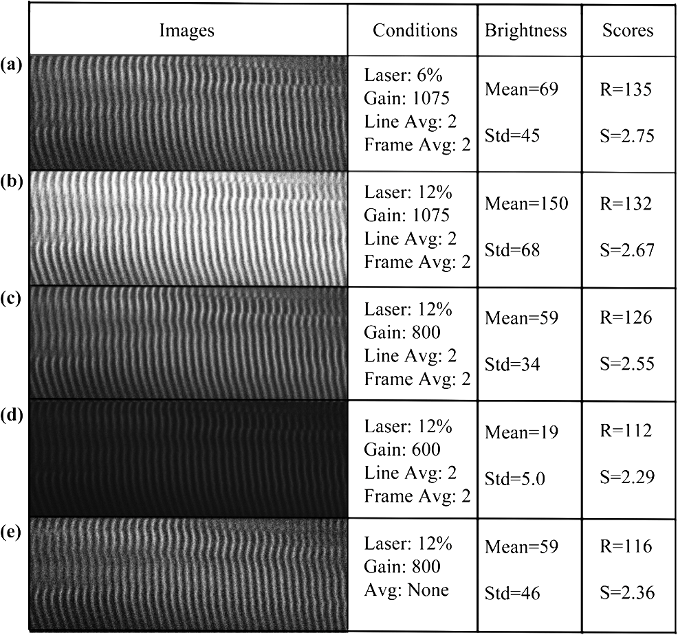

3.4.

Large Magnification Changes Affect MARS Scores

Magnification is another imaging variable that needs to be assessed, since it is sometimes necessary to compare images recorded on different instruments. The images may have been taken at slightly different magnifications (for example, with a $60 \times$ versus $63 \times$ lens without zoom compensation). To examine the effect of magnification on $R$ and $S$ , we imaged the same sample under various zooms (from $1 \times$ to $6 \times$ ) with the same $40 \times$ oil immersion objective. To make sure the same area was selected under different magnifications, we drew proportionately smaller ROIs for smaller zooms. The $R$ and $S$ scores for three different muscle fibers under different magnification are shown in Table 2. Based on $R$ and $S$ values, fiber 3 is in very good condition while fibers 1 and 2 are in relatively poor condition. The results for these three fibers (Table 2) all demonstrate a slight decline of the scores with decreased magnification. For a more graphic representation of the results, we plotted $R$ and $S$ values normalized to zoom $6 \times$ values as 100% (Fig. 6). On average, $R$ and $S$ drop by 25% when the magnification changes from $6 \times$ to $3 \times$ zoom. The decrease is not linear, and each of the images has its own curve. Whether the initial score is high or low does not make a difference. These results indicate that images taken with small magnification differences can be pooled together for MARS quantitation, but that images taken with larger differences such as $> 1.5$ -fold should not be pooled.

Table 2

R and S scores for 3 muscle samples at different magnifications with a 40× oil objective.

	Sample 1		Sample 2		Sample 3
Zoom	$R$	$S$	$R$	$S$	$R$	$S$
$6 \times$	21.9	0.438	29.3	0.569	276	4.76
$5 \times$	23.0	0.463	28.7	0.552	231	4.22
$4 \times$	21.8	0.441	22.3	0.457	244	4.48
$3 \times$	19.1	0.388	16.6	0.398	217	4.01
$2 \times$	16.8	0.350	15.3	0.410	198	3.86
$1 \times$	11.3	0.288	15.7	0.421	211	3.85

Fig. 6

$R$ and $S$ are affected by large magnification changes. Three samples with different muscle condition were imaged. To assess the effect of magnification, the same area was imaged with one objective lens ( $40 \times$ ) and six different zoom values from 1 to 6. The plots show the scores expressed in %, with the $6 \times$ magnification results taken as 100%. $R$ and $S$ decrease gradually as a function of magnification. The changes vary among different samples and are stronger between $6 \times$ and $3 \times$ (26% average decrease for $R$ ; 19% for $S$ ). The results are also presented in Table 2.

3.5.

Comparison Between R and S Scores

Both $R$ and $S$ scores are very sensitive to structural defects in muscle fibers and similarly resistant to deterioration of image quality. So far, they appear interchangeable. In order to push the comparison further, we have carried out calculations for more than 150 muscle fiber images covering a large range of conditions. $R$ and $S$ were then plotted against each other (Fig. 7). Logarithmic data were used for both scores because of the broad dynamic range. In the middle part (for $R$ values from 1000 to 10 or $S$ values from 10 to 0.1), the dots almost fall on a straight line, which is $\log S = \log R - 1.7$ , or $S \approx R / 50$ . Divergence happens at the two ends.

Fig. 7

$R$ and $S$ scores are strongly correlated. To generate this plot, all $R$ and $S$ values compiled in the present work were pooled. A logarithmic plot was used to ease the representation of the large dynamic range of values. For the middle part of the plot ( $S$ values from 10 to 0.1), the dots practically fall on a straight line which is along $\log S = \log R - 1.7$ , indicating a strong correlation. However, the distributions are scattered at the two ends, especially for fibers in very bad condition ( $S < 0.1$ ) indicating different sensitivities of $R$ and $S$ .

3.6.

MARS Successfully Highlights Differences Between Samples as well as Fiber-to-Fiber Variability

In human muscle diseases, the degree of damage varies between fibers. For example, biopsies from adult subjects with late-onset Pompe disease show normal-looking fibers next to seriously damaged ones.²³^,²⁷ This factor complicates the evaluation of a biopsy.

To test how MARS deals with such variation and whether it is able to detect differences between heterogenous samples, we collected SHG images from the following samples: (1–2) two biopsies from an infant whose genetic make-up was consistent with late-onset Pompe disease, the first biopsy taken just before starting ERT at 2.5 mo of age and the other one taken after 6 mo of ERT (Pt. NBSL15 in Ref. 30); (3) a biopsy from a 10-year-old child with a mitochondrial disease; (4) a biopsy from a healthy adult; and (5–6) samples from two wild-type mice. For each sample, a minimum of 15 SHG images were collected, each image covering one to three fibers, regardless of the degree of damage. Two to three regions of interest were selected from each image and scored with MARS.

Since $R$ and $S$ scores can differ by orders of magnitude between different fiber images [Fig. 2(a) and 2(b)], the regular average or the arithmetic mean would not be a good representation to evaluate the condition as a whole for the individual, because the higher score results would dominate the final score and the lower scores would have a much smaller impact. To have balanced contributions from both high and low scores, we used the log-average or geometric mean.

The results are presented in Fig. 8 and Table 3. Within the limited sample size of this pilot study, $R$ and $S$ scores give very similar results. For the infant with late-onset Pompe, there is a large significant increase after treatment, although a group of fibers remain at the lower scores, no better than the worst of the untreated fibers. The log-average for $R$ increases from $0.95 \pm 0.36$ to $1.52 \pm 0.43$ ( $P < 0.001$ ) and $S$ from $- 0.66 \pm 0.33$ to $- 0.14 \pm 0.41$ ( $P < 0.001$ ). Without access to true control biopsies of matched age, it is not possible to assess more exactly the respective contributions of muscle maturation and of ERT to the improvement of the scores. This was not the goal of the present study. The scores for the child and adult control subjects are significantly higher than both scores for the patient with Pompe, and the scores for the healthy adult control subject are significantly higher than those of the child control subject. Therefore, MARS has no problems detecting differences between samples, even in the presence of a large spread in the quality of the fibers. The heterogeneity of the samples is reflected in the large standard deviation. Furthermore, the two control mouse samples obtained scores in the same range as those from healthy humans, although with differences between the two of them. It will take a larger study to determine whether these differences indicate health problems in one of the animals or normal variations between animals. Such work will help determine how many images should be quantitated and how much fibers vary in healthy animals.

Fig. 8

$S$ values highlight differences in muscle condition in a variety of human and mouse samples. SHG images were collected from different human and mouse samples, as indicated below the horizontal axis. From each sample at least 35 fiber images were analyzed and plotted in KaleidaGraph. The middle line in the box represents the median and the height of the box represents the standard deviation. Since $S$ and $R$ values show very similar trends, only $S$ is displayed here.

Table 3

Log values of R and S for four human biopsies and two mouse muscle samples. Value in each cell represents the average value±standard deviation in that group.

	$Log R$	$Log S$
Pompe patient, before ERT	$0.95 \pm 0.36$	$- 0.66 \pm 0.33$
Pompe patient, before ERT	$1.52 \pm 0.43$	$- 0.14 \pm 0.41$
Child control	$1.84 \pm 0.50$	$0.15 \pm 0.46$
Adult control	$2.50 \pm 0.46$	$0.74 \pm 0.37$
Mouse control #1	$2.34 \pm 0.37$	$0.62 \pm 0.34$
Mouse control #2	$3.01 \pm 0.56$	$1.20 \pm 0.48$

4. Discussion

The software presented here, MARS, fills a void by offering an automated, quantitative analysis of light microscopy images of skeletal muscle fibers to assess conditions that can cover a wide range of defects and of damage degree.

In the analysis of muscle biopsies, it is often necessary to compare and analyze light microscopy images collected over many sessions, possibly by different microscopists. It is therefore important to understand how limited variations of imaging parameters, such as image brightness, contrast, signal-to-noise ratio, magnification, and so on, affect the analysis. We have thus carried out an analysis of the effects of several of these parameters on the results obtained by MARS.

Image brightness and contrast are largely determined by the laser power and the detector gain and offset. A histogram equalization process is applied to all images as a first step of the MARS calculations. Thus, brightness and contrast, in theory, should not impact the final scores as long as the images were collected with proper exposure, that is, without any saturation.

Images can also be affected by instrument noise and by light noise. Dark current is a small electric current that flows through detectors even when no photon is present, and it is one of the main noise sources for detectors such as CCD, PMT, and photodiode.²⁸^,²⁹ Shot noise is caused by the uncertainty of detecting one photon when small numbers of photons are present. It may be dominant in imaging with low laser power or low quantum yield from fluorophores and can be reduced by increasing the light intensity. The distribution of shot noise is a Poisson distribution, and is not very different from Gaussian noise.³¹ Impulsive noise, also called salt-and-pepper noise, is also observed in some confocal images when dead pixels are present in CCD detectors.³² To assess MARS, we have added high noise levels. For example, the 50% variance in Gaussian noise is greater than the noise level usually seen in SHG imaging, because the level of noise is so significant that any microscopist would try to adjust laser power and detector gain to achieve better images. Figure 4 and Table 1 demonstrate that the scores $R$ and $S$ are little affected by noise.

Laser power, detector gain, and averaging are commonly used in optimizing image quality in SHG. The conditions have a direct influence on the image brightness and SNR. We already demonstrated, by modifying images after acquisition, that brightness and noise level have very limited impacts on $R$ and $S$ scores. Thus, the combination of these two factors should not have a major influence either, as confirmed in Fig. 5.

Larger magnification (zoom change without numerical aperture change) usually offers finer cellular structure, slower scanning, and better signal-to-noise ratio, but at the cost of higher laser damage. The striation interval for muscle fibers is of the order of 2 μm, which is resolved by $20 \times$ or higher magnification objectives. MARS calculates the striation separation and angle at the beginning of the processing, then generates a certain number of matrices (GLCMs, as explained in Sec. 2) and calculates texture correlation for each of them. The number of matrices built in this step is directly related to the striation distance in pixels. Therefore, MARS creates more GLCMs for larger zooms. The number of data points in the texture correlation plot with a $6 \times$ zoom is 6 times the number with a $1 \times$ zoom. Fewer data points in the texture correlation plots lead to larger data fluctuation, especially when the collecting frequency is close to the Nyquist rate.³³ As a result, the periodical components decrease and both $R$ and $S$ are affected. Our analysis suggests that images differing in magnification by $2 \times$ should not be compared directly, although one could argue that a 20% to 25% change in $R$ and $S$ is not compelling considering their broad dynamic range.

We developed two different scores, $R$ and $S$ , as MARS outputs. In general the $R$ values tend to fluctuate more, especially for close to perfect striated fibers, because the calculation of $R$ uses the central peak in the frequency domain as the denominator. A striated fiber has a small central frequency peak and a small change in that value leads to significant fluctuations in $R$ . On the other hand, a severely damaged muscle fiber has a very weak signal at the first frequency peak (the numerator); in some extreme cases the peak is not detectable and consequently $R$ score becomes less accurate. $S$ score also has its own limitations, because it involves curve fitting. On some rare occasions MATLAB Curve Fitting Toolbox cannot find the best fit but generates a false minimum instead. In such cases, the factor $r$ square, which indicates how good the fit is, is a smaller number. We only use the $S$ results when the $r$ square is over 0.70. Although the fitting failure only happens occasionally (about once every 30 fibers), it could be a problem with precious biopsies. However, because of the relation $S \approx R / 50$ (see Fig. 7), we then can use $R$ score to get an estimation of $S$ value and avoid the curve-fitting step.

As discussed above, each score alone will have some occasional limitations. However, these two scores are complementary and, therefore, are more robust to handle all kinds of muscle samples. In practice, we recommend using $S$ score as the major indicator, and converting $R$ to $S$ when the curve-fitting method fails.

The only part of the software input that is not automated is the choice of the ROI to analyze. Because of the high sensitivity of the software, it is important to exclude all features that result from sample handling and mounting that could be viewed by MARS as defects. In images such as those obtained by SHG, we normally view several muscle fibers in one field of view. Each fiber must be evaluated individually since SHG images have a well-demarked interruption between neighboring fibers,²⁷ which would be considered by the software as a muscle defect. The development of a module that would automatically determine the limit of muscle fibers by taking into account another imaging modality such as phase contrast or 2-PE (2-photon emitted fluorescence) has been difficult to implement, so far. However, given the high degree of variability in muscle damage between fibers, it makes sense from a biological point of view to image ROIs for each available fiber.

MARS is robust when imaging conditions such as brightness, noise, and magnification are changed. However, sample preparation and handling, which cannot be totally controlled, must also be taken into account. We store paraformaldehyde-fixed muscle samples at $- 20 ° C$ in 50% phosphate-buffered glycerol without apparent loss of the myosin SHG signal. However, glycerol storage affects collagen SHG by causing unwinding of its triple helix structure.³⁴ Areas with damage from handling such as pinching with forceps, or making a hole with micro needles, can be identified in transmitted light and avoided. Damage such as stretching, on the other hand, may result both from manual stretching on a support before fixation, or from a disease state.¹⁹ Other imaging parameters must still be considered. For example, in thick samples the SHG signal may be reduced by absorption and diffraction. Furthermore, SHG signal is also affected by the polarization angle of the incident light.³⁵ Therefore, a standardized sample preparation and imaging procedure are needed.

Finally, MARS can be used both to estimate variability between fibers within a muscle sample, and to compare different samples, as shown in Fig. 8 and Table 3. The condition of the muscle fibers of the patient used in this study was good compared to that of patients with early onset Pompe. MARS was still able to detect a significant improvement in the muscle condition after 6 mo of ERT, in agreement with clinical observations for this patient.³⁰ However, the scores remain significantly lower than those of control subjects, because of the disease itself, because of the age difference, or because of both. Ideally, several biopsies from healthy individuals of matching age should be assessed and a “normal range” defined. For obvious ethical reasons there are no or very few open muscle biopsies from healthy infants. In the absence of such control biopsies, the best range of values was obtained from child and adult control subjects. From the data we analyzed so far, $S = 2$ and $R = 100$ (or $\log S = 0.3$ and $\log R = 2$ ) approximately mark the transition between healthy and diseased muscle. The scores for both adult and mouse controls are well above these values; the scores for the patients with Pompe before ERT well below; and the scores for the same patient after treatment and for the child control below and above, respectively, but closer to the borderline. Even for animal muscles or for healthy human muscles, we know in fact little of the variation to be expected and whether high-resolution techniques such as SHG can be diagnostic of new conditions. MARS should be helpful in this regard.

5. Conclusions

We demonstrate that MARS is highly sensitive to both subtle pattern disruptions and major interruptions in muscle fiber structures. The results from the two-score rating system show strong correlation to the muscle conditions. Our results also suggest that MARS results are robust when imaging parameters such as brightness, contrast, noise level, and magnification vary, so it is feasible to compare the scores acquired under different conditions. Except for picking up the ROI, which is done by users, MARS performs the detection and evaluation automatically. Therefore, MARS can give fast and unbiased assessment for evaluating muscle conditions regardless of the type of muscle defects. Overall we propose MARS as a robust tool to assess the condition of individual skeletal muscle fibers and also to address wider questions of muscle disease assessment.

Acknowledgments

The authors thank Drs. Kristien J. M. Zaal (NIAMS) and Christian Combs (NHLBI) for many stimulating discussions, Dr. Thorkil Ploug (Univ. of Copenhagen) for adult human muscle fibers and a reviewer for the inspiring comments. This work was supported by the Intramural Research Program of the National Institute for Arthritis and Musculoskeletal and Skin Diseases.

References

1.

R. J. TalmadgeR. R. RoyV. R. Edgerton, “Muscle fiber types and function,” Curr. Opin. Rheumatol., 5 (6), 695 –705 (1993). http://dx.doi.org/10.1097/00002281-199305060-00002 CORHES 1040-8711 Google Scholar

2.

A. J. McComas, Skeletal Muscle: Form and Function, Human Kinetics Publishers, Champaign, IL (1996). Google Scholar

3.

W. ScottJ. StevensS. A. Binder-Macleod, “Human skeletal muscle fiber type classifications,” Phys. Ther., 81 (11), 1810 –1816 (2001). POTPDY Google Scholar

4.

A. F. HuxleyR. Niedergerke, “Structural changes in muscle during contraction: interference microscopy of living muscle fibres,” Nature, 173 (4412), 971 –973 (1954). http://dx.doi.org/10.1038/173971a0 NATUAS 0028-0836 Google Scholar

5.

H. HuxleyJ. Hanson, “Changes in the cross-striations of muscle during contraction and stretch and their structural interpretation,” Nature, 173 (4412), 973 –976 (1954). http://dx.doi.org/10.1038/173973a0 NATUAS 0028-0836 Google Scholar

6.

M. A. GeevesK. C. Holmes, “Structural mechanism of muscle contraction,” Ann. Rev. Biochem., 68 (1), 687 –728 (1999). http://dx.doi.org/10.1146/annurev.biochem.68.1.687 ARBOAW 0066-4154 Google Scholar

7.

E. Ralstonet al., “Detection and imaging of non-contractile inclusions and sarcomeric anomalies in skeletal muscle by second harmonic generation combined with two-photon excited fluorescence,” J. Struct. Biol., 162 (3), 500 –508 (2008). http://dx.doi.org/10.1016/j.jsb.2008.03.010 JSBIEM 1047-8477 Google Scholar

8.

E. P. HoffmanR. H. Brown Jr.L. M. Kunkel, “Dystrophin: the protein product of the Duchenne muscular dystrophy locus,” Cell, 51 (6), 919 –928 (1987). http://dx.doi.org/10.1016/0092-8674(87)90579-4 CELLB5 0092-8674 Google Scholar

9.

B. J. Petrofet al., “Dystrophin protects the sarcolemma from stresses developed during muscle contraction,” Proc. Natl. Acad. Sci. U.S.A., 90 (8), 3710 –3714 (1993). http://dx.doi.org/10.1073/pnas.90.8.3710 PNASA6 0027-8424 Google Scholar

10.

N. Rabenet al., “Suppression of autophagy in skeletal muscle uncovers the accumulation of ubiquitinated proteins and their potential role in muscle damage in Pompe disease,” Hum. Mol. Genet., 17 (24), 3897 –3908 (2008). http://dx.doi.org/10.1093/hmg/ddn292 HMGEE5 0964-6906 Google Scholar

11.

O. Friedrichet al., “Microarchitecture is severely compromised but motor protein function is preserved in dystrophic mdx skeletal muscle,” Biophys. J., 98 (4), 606 –616 (2010). http://dx.doi.org/10.1016/j.bpj.2009.11.005 BIOJAU 0006-3495 Google Scholar

12.

D. O. Furstet al., “The organization of titin filaments in the half-sarcomere revealed by monoclonal-antibodies in immunoelectron microscopy: a map of 10 nonrepetitive epitopes starting at the Z-line extends close to the M-line,” J. Cell Biol., 106 (5), 1563 –1572 (1988). http://dx.doi.org/10.1083/jcb.106.5.1563 JCLBA3 0021-9525 Google Scholar

13.

E. RalstonT. Ploug, “Pre-embedding staining of single muscle fibers for light and electron microscopy studies of subcellular organization,” Scanning Microsc. Suppl., 10 249 –259 (1996). SCMIEU 0891-7035 Google Scholar

14.

T. Plouget al., “Analysis of GLUT4 distribution in whole skeletal muscle fibers: identification of distinct storage compartments that are recruited by insulin and muscle contractions,” J. Cell Biol., 142 (6), 1429 –1446 (1998). http://dx.doi.org/10.1083/jcb.142.6.1429 JCLBA3 0021-9525 Google Scholar

15.

R. M. WilliamsW. R. ZipfelW. W. Webb, “Interpreting second-harmonic generation images of collagen I fibrils,” Biophys. J., 88 (2), 1377 –1386 (2005). http://dx.doi.org/10.1529/biophysj.104.047308 BIOJAU 0006-3495 Google Scholar

16.

P. J. CampagnolaC. Y. Dong, “Second harmonic generation microscopy: principles and applications to disease diagnosis,” Laser Photon. Rev., 5 (1), 13 –26 (2011). http://dx.doi.org/10.1002/lpor.v5.1 1863-8880 Google Scholar

17.

M. Bothet al., “Second harmonic imaging of intrinsic signals in muscle fibers in situ,” J. Biomed. Opt., 9 (5), 882 –892 (2004). http://dx.doi.org/10.1117/1.1783354 JBOPFO 1083-3668 Google Scholar

18.

M. E. Llewellynet al., “Minimally invasive high-speed imaging of sarcomere contractile dynamics in mice and humans,” Nature, 454 (7205), 784 –788 (2008). http://dx.doi.org/10.1038/nature07104 NATUAS 0028-0836 Google Scholar

19.

S. V. Plotnikovet al., “Measurement of muscle disease by quantitative second-harmonic generation imaging,” J. Biomed. Opt., 13 (4), 044018 (2008). http://dx.doi.org/10.1117/1.2967536 JBOPFO 1083-3668 Google Scholar

20.

C. S. Garbeet al., “Automated multiscale morphometry of muscle disease from second harmonic generation microscopy using tensor-based image processing,” IEEE Trans. Biomed. Eng., 59 (1), 39 –44 (2012). http://dx.doi.org/10.1109/TBME.2011.2167325 IEBEAX 0018-9294 Google Scholar

21.

R. M. HaralickK. ShanmugaI. Dinstein, “Textural features for image classification,” IEEE Trans. Syst. Man Cybern., SMC3 (6), 610 –621 (1973). http://dx.doi.org/10.1109/TSMC.1973.4309314 Google Scholar

22.

H. TamuraS. MoriT. Yamawaki, “Textural features corresponding to visual perception,” IEEE Trans. Syst. Man Cybern., 8 (6), 460 –473 (1978). http://dx.doi.org/10.1109/TSMC.1978.4309999 Google Scholar

23.

N. RabenP. H. Plotz, “A new look at the pathogenesis of Pompe disease,” Clin. Therap., 30 (Suppl. 3), S86 –S87 (2008). http://dx.doi.org/10.1016/S0149-2918(08)00364-0 CLTHDG 0149-2918 Google Scholar

24.

N. Rabenet al., “Differences in the predominance of lysosomal and autophagic pathologies between infants and adults with Pompe disease: implications for therapy,” Mol. Genet. Metab., 101 (4), 324 –331 (2010). http://dx.doi.org/10.1016/j.ymgme.2010.08.001 MGMEFF 1096-7192 Google Scholar

25.

Y. H. Chienet al., “Pompe disease in infants: improving the prognosis by newborn screening and early treatment,” Pediatrics, 124 (6), e1116 –e1125 (2009). http://dx.doi.org/10.1542/peds.2008-3667 PEDIAU 0031-4005 Google Scholar

26.

J. Bergstrom, “Percutaneous needle-biopsy of skeletal-muscle in physiological and clinical research,” Scand. J. Clin. Lab. Invest., 35 (7), 606 –616 (1975). http://dx.doi.org/10.3109/00365517509095787 SJCLAY 0036-5513 Google Scholar

27.

E. Ralstonet al., “Detection and imaging of non-contractile inclusions and sarcomeric anomalies in skeletal muscle by second harmonic generation combined with two-photon excited fluorescence,” J. Struct. Biol., 162 (3), 500 –508 (2008). http://dx.doi.org/10.1016/j.jsb.2008.03.010 JSBIEM 1047-8477 Google Scholar

28.

D. R. Sandisonet al., “Quantitative comparison of background rejection, signal-to-noise ratio, and resolution in confocal and full-field laser scanning microscopes,” Appl. Optics, 34 (19), 3576 –3588 (1995). http://dx.doi.org/10.1364/AO.34.003576 APOPAI 1559-128X Google Scholar

29.

R. H. Webb, “Confocal optical microscopy,” Rep. Prog. Phys., 59 (3), 427 –471 (1996). http://dx.doi.org/10.1088/0034-4885/59/3/003 RPPHAG 0034-4885 Google Scholar

30.

Y. H. Chienet al., “Early pathologic changes and responses to treatment in patients with later-onset pompe disease,” Pediatr. Neurol., 46 (3), 168 –171 (2012). http://dx.doi.org/10.1016/j.pediatrneurol.2011.12.010 JPNOA7 1304-2580 Google Scholar

31.

H. QianE. L. Elson, “On the analysis of high order moments of fluorescence fluctuations,” Biophys. J., 57 (2 I), 375 –380 (1990). http://dx.doi.org/10.1016/S0006-3495(90)82539-X BIOJAU 0006-3495 Google Scholar

32.

P. P. MondalK. RajanI. Ahmad, “Filter for biomedical imaging and image processing,” J. Opt. Soc. Am. A, 23 (7), 1678 –1686 (2006). http://dx.doi.org/10.1364/JOSAA.23.001678 JOAOD6 0740-3232 Google Scholar

33.

A. J. Jerri, “The Shannon sampling theorem—its various extensions and applications: a tutorial review,” Proc. IEEE, 65 (11), 1565 –1596 (1977). http://dx.doi.org/10.1109/PROC.1977.10771 IEEPAD 0018-9219 Google Scholar

34.

S. Plotnikovet al., “Optical clearing for improved contrast in second harmonic generation Imaging of skeletal muscle,” Biophys. J., 90 (1), 328 –339 (2006). http://dx.doi.org/10.1529/biophysj.105.066944 BIOJAU 0006-3495 Google Scholar

35.

F. Vanziet al., “New techniques in linear and non-linear laser optics in muscle research,” J. Muscle Res. Cell M., 27 (5–7), 469 –479 (2006). http://dx.doi.org/10.1007/s10974-006-9084-3 JMRMD3 0142-4319 Google Scholar

© The Authors. Published by SPIE under a Creative Commons Attribution 3.0 Unported License. Distribution or reproduction of this work in whole or in part requires full attribution of the original publication, including its DOI.

Citation Download Citation

Wenhua Liu, Evelyn Ralston, and Nina Raben "Quantitative evaluation of skeletal muscle defects in second harmonic generation images," Journal of Biomedical Optics 18(2), 026005 (1 February 2013). https://doi.org/10.1117/1.JBO.18.2.026005

Published: 1 February 2013

Access the abstract

JOURNAL ARTICLE
11 PAGES

DOWNLOAD PAPER SAVE TO MY LIBRARY

GET CITATION

CITATIONS

Cited by 24 scholarly publications.

Explore citations on Lens.org

RIGHTS & PERMISSIONS

Get copyright permission Get copyright permission on Copyright Marketplace

KEYWORDS

Optical fibers

Mars

Second-harmonic generation

Biopsy

Zoom lenses

Fourier transforms

Image processing

1.

Introduction

2.

Materials and Methods