Novel registration for microcomputed tomography and bioluminescence imaging based on iterated optimal projection

Xibo Ma; Kexin Deng; Zhenwen Xue; Xueyan Liu; Shouping Zhu; Chenghu Qin; Xin Yang; Jie Tian

doi:10.1117/1.JBO.18.2.026013

6 February 2013 Novel registration for microcomputed tomography and bioluminescence imaging based on iterated optimal projection

Xibo Ma, Kexin Deng, Zhenwen Xue, Xueyan Liu, Shouping Zhu, Chenghu Qin, Xin Yang, Jie Tian

Author Affiliations +

Journal of Biomedical Optics, Vol. 18, Issue 2, 026013 (February 2013). https://doi.org/10.1117/1.JBO.18.2.026013

Abstract

As a high-sensitivity imaging modality, bioluminescence tomography can reconstruct the three-dimensional (3-D) location of an internal luminescent source based on the 3-D surface light distribution. However, we can only get the multi-orientation two-dimensional (2-D) bioluminescence distribution in the experiments. Therefore, developing an accurate universal registration method is essential for following bioluminescent source reconstruction. We can then map the multi-orientation 2-D bioluminescence distribution to the 3-D surface derived from anatomical information with it. We propose a 2-D -to-3-D registration method based on iterated optimal projection and applied it in a registration and reconstruction study of three transgenic mice. Compared with traditional registration methods based on the fixed points, our method was independent of the markers and the registration accuracy of the three experiments was improved by 0.3, 0.5, and 0.4 pixels, respectively. In addition, based on the above two registration results using the two registration methods, we reconstructed the 3-D location of the inner bioluminescent source in the three transgenic mice. The reconstruction results showed that the average error distance between the center of the reconstructed element and the center of the real element were reduced by 0.32, 0.48, and 0.39 mm, respectively.

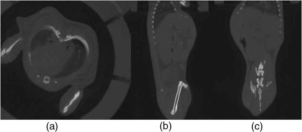
1. Introduction

In vivo bioluminescence imaging provides a high-sensitivity, low noise background, noninvasive means of monitoring genes, protein expression and other cellular events at a low cost.¹^,² However, this two-dimensional (2-D) imaging modality cannot provide three-dimensional (3-D) location information of the bioluminescent source. As a 3-D imaging modality, bioluminescence tomography (BLT) shows its advantage in determining the inner bioluminescent source distribution.³^–⁵

BLT imaging is a multi-step complex process, including multi-orientation 2-D bioluminescent images and 3-D micro-CT data acquisition, image segmentation, image registration between 2-D bioluminescent images and 3-D micro-CT volume data, and 3-D reconstruction of the bioluminescent source. Image acquisition, segmentation, registration and the reconstruction algorithm could affect the reconstruction accuracy;⁶^–⁸ among them, registration is one of the most important factors which could directly affect 3-D surface bioluminescence distribution in the experimental mouse. Therefore, we proposed a novel registration method for micro-CT and bioluminescence imaging and discussed the reconstruction accuracy based on different registration results in the following sections.

As we all know, medical image registration can be used in many aspects in preclinical and clinical studies. Maintz⁹ and his partners summarized different registration methods in detail. According to the dimension of the image space, the methods can be divided into registration between 2-D/2-D, 2-D/3-D, and 3-D/3-D. Among them, 2-D/2-D registration is currently widely used in medical imaging processing. 2-D/3-D registration is mainly used for registration between spatial data and projection data (such as CT data and x-ray data). However, for BLT, we must search for an effective method, so that data from 2-D bioluminescence data and 3-D micro-CT data could be registered between each other.

The BLT method can reconstruct the inner source distribution based on the 3-D surface bioluminescence distribution. 3-D surface bioluminescence distribution is derived by mapping the multi-orientation 2-D bioluminescence distribution onto the 3-D mouse surface based on the 2-D-to-3-D registration method. In recent years, many registration algorithms have been developed, such as Beattie’s method with the registration of planar bioluminescence to magnetic resonance and x-ray computed tomography images as a platform for the development of BLT reconstruction algorithms.¹⁰ Chandrana’s method provided a platform for coregistered ultrasound and MR contrast imaging in vivo.¹¹ Klose and his partners reconstructed the source distribution from coregistered CT and MR images and showed the performance of the coregistration method.¹² Beattie’s group provided a multimodality registration method without a dedicated multimodality scanner.¹³ Chen proposed a registration method by labeling markers on the mouse body surface which also introduced the artificial reading error of marked points.¹⁴ All of the above registration methods work depending on the system settings,. including the imaging angle of the camera and the marked points. During data acquisition, the x-ray detector and optical detector [such as the charge-coupled device (CCD) camera] must be perpendicular to each other in 3-D space. In addition, the above methods need to search the marked points on the 2-D bioluminescent images and the 3-D micro-CT images simultaneously, which will introduce random error. Therefore, it is very necessary to develop a registration method for a multi-orientation 2-D bioluminescent image and 3-D micro-CT image to facilitate biomedical research that does not depend on the system settings.

The registration between the multi-orientation 2-D bioluminescent image and 3-D micro-CT image is an important research topic that could seriously affect the accuracy of the subsequent reconstruction. In recent years, BLT has been widely used in research on the mechanisms of tumors and other diseases including bacterial infectious diseases, peripheral artery diseases and so on,¹⁵^–¹⁸ which need high reconstruction accuracy to show the minor changes at molecular and cellar levels during the process of disease progression. Many groups have proposed many algorithms on this nonrigid registration topic including affine and locally affine registration,¹⁹^,²⁰ spline-based elastic image registration,²¹ registration method based on physical model transformation²²^,²³ and so on. However, these methods have not been used in registration between a multi-orientation 2-D bioluminescent image and 3-D micro-CT image. Therefore, there was almost no systematic research on the whole process of BLT and the corresponding analysis papers with regards to the impact of registration on the reconstruction were rarely published.

In this paper, we introduce a registration method without depending on the marked points before describing the experiments in section one. Then, we apply this method on the registration between 3-D micro-CT volume data and multi-orientation 2-D bioluminescent surface of three transgenic mice. Finally, we reconstruct the inner bioluminescent source distribution of the three transgenic mice using the adaptive finite element method and evaluated the impact on reconstruction of registration deviation.

2. Experiments and Methods

2.1.

Animal Model

The transgenic mOC-Luc mice were obtained by microinjection, which harbored a luciferase marker gene under the regulation of the mouse osteocalcin (mOC) promoter. Osteocalcin (OC) is a bone tissue-specific protein expressed by osteoblasts, odontoblasts, and hypertrophic chondrocytes at the onset of tissue mineralization and it accumulates in extracellular bone. The luciferase marker gene is expressed only when the osteocalcin promoter is induced, i.e., when the cells undergo osteogenic differentiation. Transgenic mOC-Luc mice allow the investigation of OC regulation during bone remodeling and mesenchymal stem cell (MSC) osteogenic differentiation in vivo utilizing our dual-modality bioluminescent imaging system. This transgenic mouse model was kindly provided by Feng Wu of China Astronaut Research and Training Center. In this paper, we used this transgenic mouse to prove the performance of the registration method based on the iterated optimal projection and the impact of its accuracy on reconstruction.

2.2.

In Vivo Bioluminescent Image Acquisition

The in vivo white images and bioluminescent images at four orientations were acquired utilizing our dual-modality bioluminescent imaging system. The mouse was fasted overnight prior to the experiment to prevent food from interfering with the bioluminescence results. In order to compare our registration method with the registration method based on the marked points,¹⁰^,¹¹ the mouse was first injected with 200 μl urethane intraperitoneally and then was affixed to the mouse bed with marked points which was assembled on the rotation stage²⁴ (shown in Fig. 1, location 3). During bioluminescent imaging acquisition, parameters of the CCD (Princeton Instruments PIXIS 1024BR, Roper Scientific, USA) were set at $exposure time = 2 \min$ , $f - number = 2.8$ , $controller gain = 3$ , $rate = 1 MHz$ , $resolution = 16 bits$ , and $read out = low noise$ . In addition, during the white imaging acquisition, parameters of the CCD were set at the $exposure time = 10 ms$ ; the other parameters were the same as those of the bioluminescent imaging acquisition. The bioluminescent image acquisition experiments were carried out in a completely dark environment. The imaging coordinates and the corresponding pixel values were quantified from the acquired image using Windows Molecular Imaging System (WinMI) software, which was developed based on the Medical Imaging ToolKit (MITK,²⁵ Medical Image Processing and Analysis group, Institute of Automation, Chinese Academy of Sciences, Beijing, China; www.mitk.net). The four orientation white light images are shown in Fig. 2.

Fig. 1

Our prototype BLT/micro-CT dual modality imaging system. 1, CCD camera; 2, x-ray detector; 3, mouse bed; 4, x-ray tube; 5, anesthesia machine; 6, rotation stage.²⁴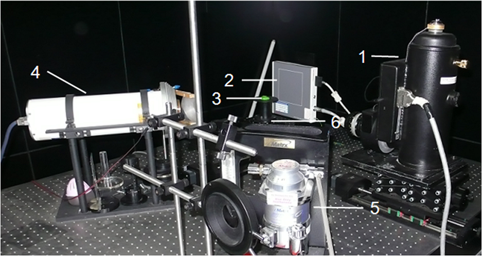

Fig. 2

Four orientation (2-D) white light images of the transgenic mouse; 0-deg., anterior-posterior; 90-deg., left lateral; 180-deg., posterior-anterior; 270-deg., right lateral image. (Green) Circles indicating the 24 marked points with No. 1 through 24.

2.3.

Micro-CT Imaging Acquisition and Reconstruction

The anatomical information of the transgenic mouse was acquired by the micro-CT system for the following registration. The micro-CT system consists of a microfocus x-ray source with a focal spot size of 30 μm, a flat-panel x-ray detector with a $1120 \times 1172 pixel$ photodiode array and a 50 μm pixel pitch (shown in Fig. 1, location 2). In the second hour after injecting 200 μl Fenestra VC into the tail vein, 500 projection views were collected in 8.5 mins. During the image acquisition, the parameter of the micro-CT was set as follows: voltage of the x-ray tube was 50 kVp, the integration time of the detector was 0.467 s, the size of each projection view was $1120 \times 1172$ , and the pixel size of the detector was $0.1 \times 0.1 {mm}^{2}$ . After acquiring the projection data, a graphics-processing-unit accelerated Feldkamp-Davis-Kress method²⁶ was used to reconstruct the volume data (shown in Fig. 3); the type was 16 bits unsigned short point and the volume size was $512 \times 512 \times 256$ . The total imaging time was 43.170 s, which included reading the data from the disk and reconstructing the volume data. Then, the 3-D surface image of the transgenic mouse was derived using the thresholding algorithm of the MITK toolkit (shown in Fig. 4).

Fig. 3

Micro-CT volume data of the transgenic mouse. (a) coronal image; (b) transectional image; (c) sagittal image.

Fig. 4

2-D projection of 3-D mouse skin surface of the transgenic mouse. 0-deg., anterior-posterior; 90-deg., left lateral; 180-deg., posterior-anterior; 270-deg., right lateral image.

2.4.

Registration Method Based on the Iterated Optimal Projection

This registration method can be divided into three steps and the corresponding flowchart of the whole algorithm is shown in Fig. 5.

Fig. 5

The flowchart of the algorithm.

In the first step, we used the Canny method to extract the mouse contour curves.²⁷^,²⁸ In this process, we used the derivative of the Gaussian function to calculate the image gradient. The input image was first convoluted with a Gaussian kernel, as shown in Eq. (1):

Eq. (1)

S (x, y) = G (x, y, σ) \times I (x, y),

where

σ

stands for the smoothness of the image which is often determined from experience,

I (x, y)

is the function of the image,

(x, y)

is the coordinate of the image, and

G (x, y; σ)

is a 2-D Gaussian function of normal distribution. Afterwards, we used the first-order finite-difference method to estimate the two arrays of the partial derivatives:

Eq. (2)

D_{x} (x, y) \approx [S (x, y + 1) - S (x, y) + S (x + 1, y + 1) - S (x + 1, y)] / 2 D_{y} (x, y) \approx [S (x, y) - S (x + 1, y) + S (x, y + 1) - S (x + 1, y + 1)] / 2 .

Finally, the image gradient can be obtained from the following two equations:

Eq. (3)

M (x, y) = \sqrt{D_{x} {(x, y)}^{2} + D_{y} {(x, y)}^{2}} θ (x, y) = \arctan [D_{y} (x, y) / D_{x} (x, y)],

where

M (x, y)

is the gradient amplitude and

θ (x, y)

is the gradient orientation. This equation demonstrates that the edge feature of the image is enhanced with the growth of the

M

value. Then, the nonmaximal value of the gradient was suppressed and the edge points were extracted using the dual-threshold method.²⁷^,²⁸ Afterwards, the edge points of the four-orientation 2-D white images in Fig. 2 were extracted using the Canny method and the four edge curves were set as

l_{1} (x_{1}, y_{1})

,

l_{2} (x_{2}, y_{2})

,

l_{3} (x_{3}, y_{3})

,

l_{4} (x_{4}, y_{4})

.

In the second step, we established two planes ( $ψ_{1}^{0}$ , $ψ_{2}^{0}$ ) perpendicular to each other as the initial mapping planes of the mouse to satisfy the following conditions:

Eq. (4)

ψ_{1}^{0} ⊥ τ, ψ_{2}^{0} τ, and ψ_{1}^{0} ⊥ ψ_{2}^{0},

where

τ

is the imaging platform almost parallel to the ground. Here,

ψ_{1}^{0}

and

ψ_{2}^{0}

are the planes parallel to the 0-deg. surface and 90-deg. surface in Fig. 2 which were chosen manually as the initial mapping planes. Then, the 3-D mouse surface (shown in Fig. 4) could be projected onto the two planes

ψ_{1}^{0}

,

ψ_{2}^{0}

. The 3-D mouse surfaces after projection were, respectively set as

φ_{1}

,

φ_{2}

,

φ_{3}

,

φ_{4}

, which corresponded to the four-orientation 2-D images in Fig. 2. Similarly, the edge points of

φ_{1}

,

φ_{2}

,

φ_{3}

,

φ_{4}

were extracted using the Canny method, and then the edge curves were set as

L_{1} (X_{1}, Y_{1})

,

L_{2} (X_{2}, Y_{2})

,

L_{3} (X_{3}, Y_{3})

,

L_{4} (X_{4}, Y_{4})

, respectively.

In the third step, the two curves were shifted to the same coordinate system. In order to determine the similarity of the two curves, we built a similar discriminant function:

Eq. (5)

{}^{j}F = {‖ Y_{k i} - y_{k i} ‖}_{1} = \sum_{i = 1}^{n} | Y_{k i} - y_{k i} |, X_{k i} = x_{k i}, k = 1, 2, 3, 4,

where

j

is the number of iterations. (

x_{k i}

,

y_{k i}

) is the coordinate of the edge points of the four-orientation 2-D image of the transgenic mouse and

k = 1

, 2, 3, 4 especially for the four orientations including 0-deg., 90-deg., 180-deg., and 270-deg. (

X_{k i}

,

Y_{k i}

) is the coordinate of the 2-D projection of the 3-D mouse skin surface. If

x_{k i} \neq X_{k i}

, we can get

X_{k i}^{'}

which satisfies

x_{k i} = X_{k i}^{'}

through interpolation. In

\pm 30

orientations where the iteration step is

Δ

, the initial mapping plane (

ψ_{1}^{0}

,

ψ_{2}^{0}

) was rotated and we attained a series of mapping planes (

ψ_{1}^{m}

,

ψ_{2}^{m}

),

m = 0, 1, 2 \dots

. Thus, we can get the minimum discriminant function value

{}^{1}F

and the optimal mapping plane (

ψ_{1}^{A}

,

ψ_{2}^{A}

). In the second round of the search, (

ψ_{1}^{A}

,

ψ_{2}^{A}

) was set as the initial mapping plane and the rotation angle was limited in the

\pm 30 / 2

orientation with the iteration step

Δ / 2

. After this research, we could get another minimum discriminant function value

{}^{1}F

. In the process of the iteration calculation, if

({}^{(j + 1)}F - {}^{j}F) / {}^{j}F

was less than 0.01, then iteration was terminated. If

({}^{(j + 1)}F - {}^{j}F) / {}^{j}F

was more than 0.01, then the iteration continued with the rotation orientation

\pm 30 / 2^{j - 1}

and the iteration step

Δ / 2^{j - 1}

(

j = 1, 2 \dots

).

With the above calculation, the four orientation white light images in Fig. 2 could be registered to the 3-D mouse surfaces derived from the microCT volume data. Furthermore, we could get the 3-D surface bioluminescence distribution of the transgenic mouse using the registration method based on the iterated optimal projection (shown in Fig. 6) for the following BLT.

Fig. 6

The 3-D bioluminescence distribution of transgenic mouse 1 after mapping based on the registration results using our registration method. 0-deg, anterior-posterior; 90-deg, left lateral; 180-deg, posterior-anterior; 270-deg, right lateral image.

2.5.

Three-Dimensional Reconstruction of the Inner Source Based on the Registration

Since the experiment was carried out in a totally dark environment, the propagation of bioluminescent photons in the highly-scattering biological tissues could be represented by the steady-state diffusion equation in BLT:⁷^,²⁹

Eq. (6)

- \nabla \cdot [D (x) \nabla Φ (x)] + μ_{a} (x) Φ (x) = S (x) (x \in Ω) .

The boundary condition can be depicted as

Eq. (7)

Φ (x) + 2 A (x; n, n^{'}) D (x) [v (x) \cdot \nabla Φ (x)] = 0 (x \in \partial Ω),

where

Ω

and

\partial Ω

are the domain and its boundary, respectively;

Φ (x)

denotes the photon flux density [

Watts / {mm}^{2}

];

S (x)

is the source energy density [

Watts / {mm}^{3}

];

μ_{a} (x)

is the absorption coefficient [

{mm}^{- 1}

];

D (x) = 1 / 3 [μ_{a} (x) + (1 - g) μ_{s} (x)]

is the optical diffusion coefficient [mm];

μ_{s} (x)

is the scattering coefficient [

{mm}^{- 1}

];

g

is the anisotropy parameter; and

ν

is the unit outer normal in

\partial Ω

.

In recent years, many algorithms have been developed to reconstruct the inner bioluminescent source,⁶^,³⁰^–³² which were proven to be confident in bioluminescent tomography experiments not only on phantom models but also on mouse models. Here, we chose the most commonly used adaptive finite element method (FEM) to assess the impact of registration accuracy on reconstruction using the three transgenic mice. Based on FEM, the diffusion equation could be finally transformed to

Eq. (8)

{AS}^{P} = Φ^{m} .

2.6.

Ex Vivo Validation Experiment

In the following reconstruction analysis, we used the elements in the bone nearest to the reconstructed element as the real elements to calculate the reconstruction error. In order to evaluate the feasibility of this method in the transgenic mice osteocalcin study, we designed a set of ex vivo experiments to support the reconstruction results. According to the distance between the real element and the nearest arthrosis derived from the reconstruction results, we euthanized the mice and cut the bones at different locations. The bone cells were extracted overnight using the enzymes and the bioluminescent intensity was detected using the chemiluminescence apparatus after adding enough luciferin. A detailed experimental procedure is as follows:

1. Euthanized the mice and cut the bones nearest from the reconstructed elements at different locations according to the reconstruction results.
2. Milled the bone tissue into powder using liquid nitrogen.
3. Added 0.5 ml passive lysates per 0.1 g tissue, slowly rotating for 30 min at room temperature in order to make cell cleavage adequate.
4. Centrifuged for 1 min at 12,000 rpm, and added it to the white detection plate after removing 25 μl supernatant.
5. Detected the bioluminescence intensity for 10 s after adding 50 μl luciferin (Biotium Inc., USA).

3. Results

3.1.

Registration Results

Based on this method, the 3-D mouse surfaces were mapped into four-orientation 2-D planes using the orthographic projection. According to this method, the mouse surfaces were mapped onto two planes $[(ψ_{1}^{j}, ψ_{2}^{j}), j = 0, 1, 2 \dots]$ , respectively so we could obtain four-orientation mouse surface images.

In our experiments, according to the experimental and evaluation results, the primary parameter $σ = 1.8$ which controls the size of the Gaussian kernel of the filter fit our applications the best. In order to compare our registration method with the registration method based on the marked points,¹⁰^,¹¹ the mouse was affixed to the mouse bed with marked points (shown in Fig. 2). According to the requirements of this method, the mouse must rotate along the axis without deviation during the whole experiment. Nine holes with a 1 mm diameter in the mouse bed were set as the registration points for this method. During the process of registration based on the marked points, we had to manually search the registration points of the four orientation bioluminescent images and the 3-D Micro-CT image, and validate the matching relationship of the points between the two modalities. The registration error was calculated by

Eq. (9)

RE = \sqrt{Ψ} = \sqrt{\frac{1}{N} \sum_{i = 1}^{N} [{(x_{m}^{i} - x_{B}^{i})}^{2} + {(y_{m}^{i} - y_{B}^{i})}^{2}]},

where (

x_{m}

,

y_{m}

) is the coordinate of the marked points in the 2-D bioluminescent images which are considered to be the true value in the experiment, and (

x_{B}

,

y_{B}

) is the coordinate of the corresponding marked points (

x_{m}

,

y_{m}

) which are considered to be the calculated value in the registration method. In the experiments, due to the occlusion of the marked points in the mouse bed, we cannot read the coordinates of all marked points. Here, we chose 24 marked points from the four angles to evaluate the registration accuracy (shown in Fig. 2). Among them, points 1 through 6 were on the 0 orientation surface of the mouse bed, points 7 through 12 were on the 90 orientation surface of the mouse bed, points 13 through 17 were on the 180 orientation surface of the mouse bed, and points 18 through 24 were on the 270 orientation surface of the mouse bed. Then, we could obtain the registration points of the 24 marked points on the 3-D image derived from the Micro-CT volume data corresponding to the 24 marked points on the four orientation 2-D white images of the transgenic mouse using the two registration methods. The coordinates of the 24 marked points on the mouse bed were considered to be more accurate than the points marked on the mouse because of the rigidity characteristics of the mouse bed.

According to the above error calculation equation, we could get the registration deviation between the points on the 3-D image and the points on the four orientation 2-D images using the two registration methods. Based on the registration results, we could also calculate the average registration deviation of the marked points at every angle and the total average deviation of all 24 marked points. The results are shown in Table 1. Meanwhile, in order to show the registration deviation of the two registration methods, we made the 24 marked points and their registration points using the two registration methods in a coordinate system (shown in Fig. 7). From the figure, we could also find that the registration deviation of our method was less than the registration deviation of Beattie’s and Chandrana’s methods.¹⁰^,¹¹

Table 1

The registration results of three mice using the two registration methods.

Mouse	Method	$0 \deg$	$90 \deg$	$180 \deg$	$270 \deg$	Average deviation
Mouse 1	IOP	2.2 pixels	2.7 pixels	2.1 pixels	2.6 pixels	2.4 pixels
Mouse 1	MP	1.7 pixels	2.6 pixels	3.5 pixels	2.9 pixels	2.7 pixels
Mouse 2	IOP	1.9 pixels	2.5 pixels	2.3 pixels	2.2 pixels	2.2 pixels
Mouse 2	MP	2.8 pixels	2.7 pixels	2.2 pixels	2.9 pixels	2.7 pixels
Mouse 3	IOP	2.3 pixels	2.4 pixels	2.5 pixels	2.4 pixels	2.4 pixels
Mouse 3	MP	3.5 pixels	2.8 pixels	1.9 pixels	2.9 pixels	2.8 pixels

Note: IOP stands for the registration results of three mice using our registration methods based on the iterated optimal projection; MP stands for the registration results of three mice using the registration algorithm based on the marked points.10,11

Fig. 7

Coordinates of the 24 marked points and coordinates of their registration points using the two registration methods; points A stand for the 24 marked points; points B stand for the registration points of the 24 marked points using our registration method, and points C stand for the registration points of the 24 marked points using Beattie’s and Chandrana’s methods.¹⁰^,¹¹

With these experiments, we found that the average registration deviation using the registration method based on the marked points¹⁰^,¹¹ was 2.7 pixels and the average registration deviation using our registration method based on the iterated optimal projection was 2.4 pixels. For this experiment, the pixel of our CCD was 0.02 mm, and the magnification of our imaging system was 4.5. Therefore, the average absolute registration deviations of the two methods were 0.24 and 0.22 mm, respectively. The results showed that the registration method based on the iterated optimal projection could improve the registration accuracy by 0.02 mm (0.3 pixels).

In addition, in order to evaluate the stability of the algorithm, the experiments were carried out on another two mice, and the registration results are shown in Table 1. The results showed that the average registration deviation of mouse 2 using the two methods was 2.2 pixels (0.20 mm) and 2.7 pixels (0.24 mm), respectively and the average registration deviation of mouse 3 using the two methods was 2.4 pixels (0.22 mm) and 2.8 pixels (0.25 mm), respectively. In contrast with the registration method based on the marked points,¹⁰^,¹¹ our method could improve the average registration deviation by 0.5 pixels (0.04 mm) and 0.4 pixels (0.03 mm).

At the same time, in order to evaluate the performance of the algorithm, the dispersion coefficient was used to show the representativeness of the total registration deviation. Here, we used the coefficient of variance to represent the dispersion coefficient. The equation is shown as follows:

Eq. (10)

DC = \frac{\sqrt{\sum_{i = 1}^{N} {[{AD}_{i} - \bar{AD}]}^{2}}}{\bar{AD}} (N = 4),

where DC is the dispersion coefficient, AD is the average registration deviation at four angles, and

\bar{AD} = {AD}_{i} / 4

,

i = 1

, 2, 3, 4. According to the equation, we could obtain the dispersion coefficient results of the three mice using the two registration methods; the results are shown in Table 2. The results showed that the average dispersion coefficient using the two registration methods was 0.07 and 0.40 pixels, respectively. The high dispersion coefficient (DC) of the registration method based on the marked points means the DC at the four angles is obviously different. All of these results showed that our registration method was more stable than the registration method based on the marked points.¹⁰^,¹¹

Table 2

Dispersion coefficient (DC) for the registration deviation of the three mice using the two registration methods.

DC	Mouse 1	Mouse 2	Mouse 3	Average DC
DC1	0.11	0.09	0.01	0.07
DC2	0.63	0.11	0.47	0.40

Note: DC1 (dispersion coefficient 1) stands for the dispersion coefficient of the registration deviation using our registration method based on the iterated optimal projection; DC2 (dispersion coefficient 2) stands for the dispersion coefficient of the registration deviation using the registration methods based on the marked points.10,11

Furthermore, the bioluminescence distribution derived from the four-orientation 2-D images was mapped onto the 3-D surface of the mouse derived from the Micro-CT image using our registration method based on the iterated optimal projection. The 3-D bioluminescence distribution of transgenic mouse 1 after mapping based on the registration results using our registration method is shown in Fig. 6. The distribution of the bioluminescent source can be calculated through an FEM method. In the next section, we will discuss the impact on reconstruction of registration deviation in more detail.

3.2.

Reconstruction Analysis Based on Registration

In order to evaluate the impact on the reconstruction results of the registration deviation, we reconstructed the inner bioluminescent source distribution using the above FEM method with the same parameters. In addition, we used a bioluminescence decay calibration strategy to reduce the impact on the reconstruction of bioluminescence decay.²⁴

According to the reconstructed volume data from Micro-CT, the transgenic mouse was segmented into two major organs to represent the heterogeneous mouse, including muscle and bone. The optical properties for each organ were determined with the inverse adding doubling scheme,³³ as listed in Table 3. The reconstruction processor was run based on the parameters of the two tissues. The micro-CT volume data of the transgenic mouse was discretized into 4038 points and 20158 tetrahedrons.

Table 3

Optical parameters for different heterogeneous mouse tissues.

Material	$μ_{a} ({mm}^{- 1})$	$μ_{s} ({mm}^{- 1})$	$g$
Muscle	0.010	4.000	0.900
Bone	0.002	20.000	0.900

Note: ED1 (error distance 1) stands for the error distance between the reconstructed center of the reconstructed element and the real center of the real element of mouse 1 using the FEM method based on our registration results; ED2 (error distance 2) stands for the error distance between the reconstructed center of the reconstructed element and the real center of the real element of mouse 1 using the FEM method based on Beattie’s and Chandrana’s methods.10,11

In order to induce the ill-posedness of reconstruction, we adopted a permissible source region strategy. According to the bioluminescence distribution on the surface after mapping and bioluminescence calibration, the permissible source region (PS) was set to

Eq. (11)

PS = [(x, y, z) | 14 < x < 40, 8 < y < 28, 62 < z < 72; (x, y, z) \in Ω] .

The regularization parameter was set to

0.5 \times 10^{- 12}

and the threshold was set to 0.5. The reconstruction time of mouse 1 was 1345.6 s. Based on the heterogeneity of the mouse, the multi-bioluminescent sources in the transgenic mOC-Luc mouse were reconstructed. The reconstruction results for mouse 1 based on our registration results are shown in Fig. 8. Since the two figures were not easily distinguishable with the naked eye, the reconstruction results based on the registration results using Beattie’s and Chandrana’s methods¹⁰^,¹¹ are not shown in this paper. Here, the bioluminescent source whose intensity was less than half of the highest intensity of the bioluminescent source is not shown in the figure.

Fig. 8

Reconstructed bioluminescent source results based on our registration results; A, anterior-posterior; B, left lateral; C, posterior-anterior; D, right lateral image; E, three-dimensional reconstructed bioluminescent source.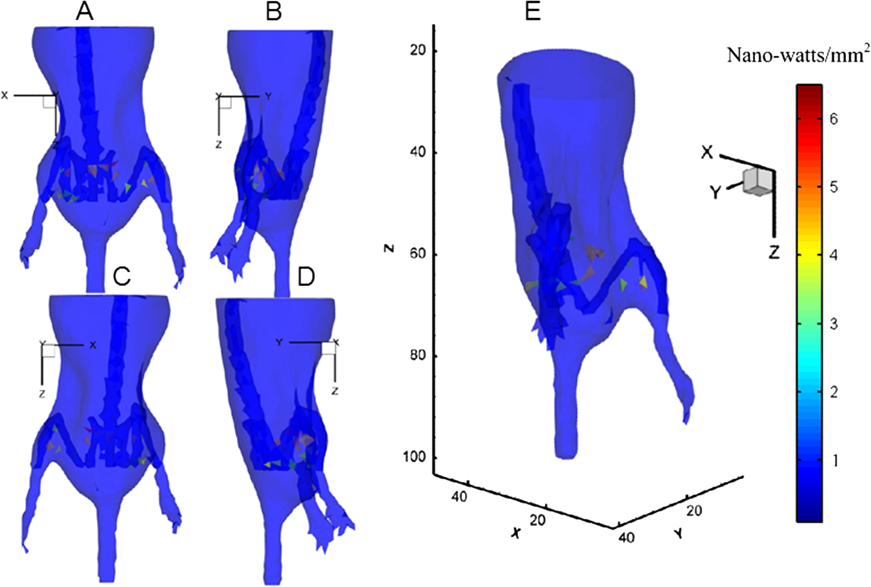

In addition, in order to assess the reconstruction accuracy, we calculated the reconstructed center of every reconstructed element. The elements in the bone nearest to the reconstructed element were considered to be the real elements. Then, the error distance (ED) could be calculated through the following equation:³⁴

Eq. (12)

ED = \sqrt{{(x_{1} - x_{2})}^{2} + {(y_{1} - y_{2})}^{2} + {(z_{1} - z_{2})}^{2}},

where (

x_{1}

,

y_{1}

,

z_{1}

) is the center of the real element, and (

x_{2}

,

y_{2}

,

z_{2}

) is the reconstructed center of the reconstructed element. The corresponding quantitative reconstruction results using the FEM method based on the two registration results are shown in Table 4.

Table 4

The error distance between the reconstructed center of the reconstructed element and the real center of the real element of mouse 1 using the FEM method based on the two registration results.

Point No.	ED1	ED2
1	1.53	1.70
2	1.71	1.69
3	1.08	1.42
4	2.48	1.99
5	0.77	2.97
6	1.22	1.62
7	1.24	1.51
8	0.85	1.36
9	1.62	1.30
10	0.97	1.27
11	1.96	3.27
12	2.81	2.02
13	1.79	1.91
14	0.83	1.21
15	1.59	1.63
16	2.39	2.57
17	0.90	1.10
18	1.10	1.51
19	1.44	2.29

According to the ex vivo validation experiments, we acquired the bone cells from six different locations and measured the bioluminescent intensity using the chemiluminescence apparatus. Based on the two bioluminescent intensity results derived from the measurement of the chemiluminescence apparatus and 3-D reconstructions, we calculated the correlation. A robust linear correlation between the two bioluminescent intensity results was observed and the corresponding results are shown in Fig. 9. The experimental results demonstrated that the evaluation method of reconstruction is effective in osteocalcin research of transgenic mice.

Fig. 9

Correlation between the two bioluminescent intensity results derived from the chemiluminescence apparatus and reconstruction. Linear regression analysis indicated a high correlation between the two bioluminescent intensity results ( $R^{2} = 0.98$ ; $p < 0.0001$ ).

Meanwhile, we had reconstructed the bioluminescence distribution of the other two mice based on the two registration results with the same parameters. We calculated the average error distance between the center of the reconstructed element and the center of the real element based on the two registration results. The results are shown in Table 5. In Table 5, “A” (mm) means the average error distance between the center of the reconstructed element and the center of the real element based on the registration results using our registration method; “B” (mm) means the average error distance between the center of the reconstructed element and the center of the real element based on the registration results using Beattie’s and Chandrana’s registration methods.¹⁰^,¹¹ The results showed that the reconstructed error distance based on the registration results using our method could be reduced by 0.32, 0.48 and 0.39 mm, respectively. From Tables 1 and 5, we found that the reconstructed error distances of the three mice were reduced by 0.16 mm (0.48 through 0.32 mm), while the registration deviation of the three mice was reduced from 0.3 pixels (0.027 mm) to 0.5 pixels (0.045 mm) demonstrating that the improvement of the reconstruction accuracy was consistent with the narrowing of the registration deviation.

Table 5

The average error distance between the center of the reconstructed element and the center of the real element based on the two registration results of the three mice.

	Mouse 1	Mouse 2	Mouse 3
A (mm)	1.49	1.36	1.56
B (mm)	1.81	1.84	1.95

4. Conclusion and Discussion

In this paper, through the registration and reconstruction experiments, we have shown that the registration deviation of the three mice was reduced by 0.3 pixels (0.027 mm), 0.5 pixels (0.045 mm) and 0.4 pixels (0.036 mm), respectively; the average error distance between the center of the reconstructed element and the center of the real element of the three mice was reduced by 0.32, 0.48, and 0.39 mm, respectively with the same reconstruction conditions and parameters. The improvement of the registration accuracy would improve the reconstruction accuracy. In the follow-up studies, we will carry out the research on an accurate and rapid registration and reconstruction method, which will achieve an automatic registration and reconstruction function. This research will be expected to facilitate the mechanistic study on the diseases of bones such as osteoporosis and hyperosteogeny through 3-D bioluminescence reconstruction of osteocalcin. Furthermore, it will promote accurate diagnosis of tumors at an early stage and the application of optical molecular imaging in clinical surgical navigation. In addition, we will attempt to study the global automatic algorithm of the whole process of BLT, which will promote the application of optical molecular imaging in clinical and preclinical oncology and drug research.

The registration method proposed in this paper avoided manual research for the fiducial markers in a Micro-CT image and four orientation bioluminescent images, which greatly reduced the introduction of random error. In the process of searching points for the registration method based on the marked points,¹⁰^,¹¹ the matching relationship between the two modalities is fuzzy and needs to be validated according to practices which would cost too much time. However, during the process of our registration method, the movement of the mouse with the bed is not restricted which made the experiments more flexible especially for continuous long-term observation of the tumor. Alternatively, the registration method based on the iterated optimal projection is robust and does not need any contrasting agent.

The main limitation of the procedure we proposed is that the mouse was required to be anesthetized during the imaging experiment. Thus, for example, registrations between functional images (or anatomical images) acquired serially over the observation course of several days could not be conducted following these procedures alone because of different conditions of the mouse after anesthesia. However, the existence of an accurately registered structural (magnetic resonance imaging-MRI, CT) image associated with each day’s functional image in many cases will fill such a serial registration gap.³⁵

In the future, we will attempt to study some registration methods without the need of mouse anesthesia, which depends on the progress of computational mathematics, optics and the improvement of medical imaging devices. Alternatively, we will study the fuzzy registration method in order to fulfill the continuous long-term observation without needing high accuracy registration, such as the observation of tumor metastasis and other disease progression. Furthermore, we will also study the impact of registration on bioluminescence reconstruction based on current research and promote the application of this method in registrations between other imaging modalities including MRI and PET. In conclusion, all of the above research will promote the development of the life science field and potentially influence other disciplines such as molecular biology, biochemistry, computational mathematics, optics and medical imaging devices.

Acknowledgments

This research is supported by the National Basic Research Program of China (973 Program) under Grant No. 2011CB707700, the National Natural Science Foundation of China under Grant Nos. 81227901, 61231004, 81071205, 81101095, 81027002, the Beijing Natural Science Foundation under Grant No. 4111004, Youth Innovation Promotion Association of CAS, the Fellowship for Young International Scientists of the Chinese Academy of Sciences under Grant No. 2010Y2GA03, and the Chinese Academy of Sciences Visiting Professorship for Senior International Scientists under Grant No. 2010T2G36. The authors would like to thank Feng Wu of China Astronaut Research and Training Center for kindly providing transgenic mice. The authors would also like to thank Dr. Karen M. von Deneen for the helpful revision of the manuscript.

References

1.

R. WeisslederV. Ntziachristos, “Shedding light onto live molecular targets,” Nat. Med., 9 (1), 123 –128 (2003). http://dx.doi.org/10.1038/nm0103-123 1078-8956 Google Scholar

2.

V. Ntziachristoset al., “Looking and listening to light: the evolution of whole-body photonic imaging,” Nat. Biotechnol., 23 (3), 313 –320 (2005). http://dx.doi.org/10.1038/nbt1074 NABIF9 1087-0156 Google Scholar

3.

X. B. Maet al., “Research on liver tumor proliferation and angiogenesis based on multi-modality molecular imaging,” Acta Biophys. Sin., 27 (4), 355 –364 (2011). http://dx.doi.org/10.3724/SP.J.1260.2011.00355 1000-6737 Google Scholar

4.

A. J. Chaudhariet al., “Hyperspectral and multispectral bioluminescence optical tomography for small animal imaging,” Phys. Med. Biol., 50 (23), 5421 –5441 (2005). http://dx.doi.org/10.1088/0031-9155/50/23/001 PHMBA7 0031-9155 Google Scholar

5.

Y. Luet al., “In vivo mouse bioluminescence tomography with radionuclide-based imaging validation,” Mol. Imaging Biol., 13 (1), 53 –58 (2011). http://dx.doi.org/10.1007/s11307-010-0332-y 1536-1632 Google Scholar

6.

Y. Lvet al., “A multilevel adaptive finite element algorithm for bioluminescence tomography,” Opt. Express, 14 (18), 8211 –822 (2006). http://dx.doi.org/10.1364/OE.14.008211 OPEXFF 1094-4087 Google Scholar

7.

W. Conget al., “Practical reconstruction method for bioluminescence tomography,” Opt. Express, 13 (18), 6756 –6771 (2005). http://dx.doi.org/10.1364/OPEX.13.006756 OPEXFF 1094-4087 Google Scholar

8.

X. Heet al., “Sparse reconstruction for quantitative bioluminescence tomography based on the incomplete variables truncated conjugate gradient method,” Opt. Express, 18 (24), 24825 –24839 (2010). http://dx.doi.org/10.1364/OE.18.024825 OPEXFF 1094-4087 Google Scholar

9.

J. B. A. MaintzM. A. Viergever, “A survey of medical image registration,” Med. Image Anal., 2 (1), 1 –36 (1998). http://dx.doi.org/10.1016/S1361-8415(01)80026-8 MIAECY 1361-8415 Google Scholar

10.

B. J. Beattieet al., “Registration of planar bioluminescence to magnetic resonance and x-ray computed tomography images as a platform for the development of bioluminescence tomography reconstruction algorithms,” J. Biomed. Opt., 14 (2), 024045 (2009). http://dx.doi.org/10.1117/1.3120495 JBOPFO 1083-3668 Google Scholar

11.

C. Chandranaet al., “Development of a platform for co-registered ultrasound and MR contrast imaging in vivo,” Phys. Med. Biol., 56 (3), 861 –877 (2011). http://dx.doi.org/10.1088/0031-9155/56/3/020 PHMBA7 0031-9155 Google Scholar

12.

A. D. KloseB. J. Beattie, “Bioluminescence tomography with CT/MRI co-registration,” in 31st Annual International Conference of the IEEE EMBS, (2009). Google Scholar

13.

B. Beattieet al., “Multimodality registration without a dedicated multimodality scanner,” Mol. Imag., 6 (2), 108 –120 (2007). MIOMBP 1535-3508 Google Scholar

14.

X. Chenet al., “Mapping of bioluminescent images onto CT volume surface for dual-modality BLT and CT imaging,” J. X-Ray Sci. Technol., 20 (1), 31 –44 (2012). http://dx.doi.org/10.3233/XST-2012-0317 JXSTE5 0895-3996 Google Scholar

15.

A. J. Minnet al., “Distinct organ-specific metastatic potential of individual breast cancer cells and primary tumors,” J. Cli. Invest., 115 (1), 44 –55 (2005). http://dx.doi.org/10.1172/JCI200522320 JCINAO 0021-9738 Google Scholar

16.

W. Wanget al., “Acridine derivatives activate p53 and induce tumor cell death through bax,” Cancer Biol. Ther., 4 (8), 893 –398 (2005). http://dx.doi.org/10.4161/cbt CBTAAO 1538-4047 Google Scholar

17.

S. M. Burnset al., “Revealing the spatiotemporal patterns of bacterial infectious diseases using bioluminescent pathogens and whole body imaging,” Contrib. Microbiol., 9 71 –88 (2001). http://dx.doi.org/10.1159/000060392 CMIMBF 0301-3081 Google Scholar

18.

E. A. Koenet al., “Molecular imaging of bone marrow mononuclear cell survival and homing in murine peripheral artery disease,” JACC Cardiovasc. Imag., 5 (1), 46 –55 (2012). http://dx.doi.org/10.1016/j.jcmg.2011.07.011 Google Scholar

19.

J. FeldmarN. Rigid, “Affine and locally affine registration of free-form surfaces,” Int. J. Comput. Vision, 18 (2), 99 –119 (1996). http://dx.doi.org/10.1007/BF00054998 IJCVEQ 0920-5691 Google Scholar

20.

V. Arsignyet al., “A Log-Euclidean polyaffine framework for locally rigid or affine registration,” Lect. Notes Comput. Sci., 4057 120 –127 (2006). http://dx.doi.org/10.1007/11784012_15 LNCSD9 0302-9743 Google Scholar

21.

K. RohrM. FornefettH. Stiehl, “Spline-based elastic image registration: integration of landmark errors and orientation attributes,” Comput. Vis. Image Und., 90 (2), 153 –168 (2003). http://dx.doi.org/10.1016/S1077-3142(03)00048-1 CVIUF4 1077-3142 Google Scholar

22.

C. Davatzikos, “Spatial transformation and registratin of brain images using elastically deformable models,” Comput. Vis. Image Und., 66 (2), 207 –222 (1997). http://dx.doi.org/10.1006/cviu.1997.0605 CVIUF4 1077-3142 Google Scholar

23.

W. CrumC. TannerD. Hawkes, “Anisotropic multi-scale fluid registration: evaluation in magnetic resonance breast imaging,” Phys. Med. Biol., 50 (21), 51 –53 (2005). http://dx.doi.org/10.1088/0031-9155/50/21/014 PHMBA7 0031-9155 Google Scholar

24.

X. B. Maet al., “Early detection of liver cancer based on bioluminescence tomography,” Appl. Opt., 50 (10), 1389 –1395 (2011). http://dx.doi.org/10.1364/AO.50.001389 APOPAI 0003-6935 Google Scholar

25.

J. TianJ. XueY. Dai, “A novel software platform for medical image processing and analyzing,” IEEE Trans. Inform. Technol. Biomed., 12 (6), 800 –812 (2008). http://dx.doi.org/10.1109/TITB.2008.926395 ITIBFX 1089-7771 Google Scholar

26.

G. R. Yanet al., “Fast cone beam CT image reconstruction using GPU hardware,” J. X-Ray Sci. Technol., 16 (4), 225 –234 (2008). JXSTE5 0895-3996 Google Scholar

27.

J. Canny, “A computational approach to edge detetion,” IEEE Trans. Pattern Anal. Mach. Intell., 8 (6), 679 –698 (1986). http://dx.doi.org/10.1109/TPAMI.1986.4767851 Google Scholar

28.

F. A. PellegrinoW. VanzellaV. Torre, “Edge detection revisited,” IEEE Trans. Syst. Man Cybern. B Cybern., 34 (3), 1500 –1518 (2004). http://dx.doi.org/10.1109/TSMCB.2004.824147 ITSCFI 1083-4419 Google Scholar

29.

M. Schweigeret al., “The finite element method for the propagation of light in scattering media; boundary and source conditions,” Med. Phys., 22 (11), 1779 –1792 (1995). http://dx.doi.org/10.1118/1.597634 MPHYA6 0094-2405 Google Scholar

30.

J. C. Fenget al., “Three-dimensional bioluminescence tomography based on Bayesian approach,” Opt. Express, 17 (19), 16834 –16848 (2009). http://dx.doi.org/10.1364/OE.17.016834 OPEXFF 1094-4087 Google Scholar

31.

K. Liuet al., “A fast bioluminescent source localization method based on generalized graph cuts with mouse model validations,” Opt. Express, 18 (4), 3732 –3745 (2010). http://dx.doi.org/10.1364/OE.18.003732 OPEXFF 1094-4087 Google Scholar

32.

B. Zhanget al., “A trust region method in adaptive finite element framework for bioluminescence tomography,” Opt. Express, 18 (7), 6477 –6491 (2010). http://dx.doi.org/10.1364/OE.18.006477 OPEXFF 1094-4087 Google Scholar

33.

S. A. PrahlV. GemertA. J. Welch, “Determining the optical properties of turbid media by using the adding doubling method,” Appl. Opt., 32 (4), 559 –568 (1993). http://dx.doi.org/10.1364/AO.32.000559 APOPAI 0003-6935 Google Scholar

34.

X. B. Maet al., “Three-dimensional multi bioluminescent sources reconstruction based on adaptive finite element method,” Proc. SPIE, 7965 79650B (2011). http://dx.doi.org/10.1117/12.878049 PSISDG 0277-786X Google Scholar

35.

K. J. Fristonet al., “Statistical parametric maps in functional imaging: a general linear approach,” Hum. Brain Mapp., 2 (4), 189 –210 (1994). http://dx.doi.org/10.1002/hbm.v2:4 HBRME7 1065-9471 Google Scholar

CC BY: © The Authors. Published by SPIE under a Creative Commons Attribution 4.0 Unported License. Distribution or reproduction of this work in whole or in part requires full attribution of the original publication, including its DOI.

Citation Download Citation

Xibo Ma, Kexin Deng, Zhenwen Xue, Xueyan Liu, Shouping Zhu, Chenghu Qin, Xin Yang, and Jie Tian "Novel registration for microcomputed tomography and bioluminescence imaging based on iterated optimal projection," Journal of Biomedical Optics 18(2), 026013 (6 February 2013). https://doi.org/10.1117/1.JBO.18.2.026013

Published: 6 February 2013

Access the abstract

JOURNAL ARTICLE
10 PAGES

DOWNLOAD PAPER SAVE TO MY LIBRARY

GET CITATION

CITATIONS

Cited by 6 scholarly publications.

Explore citations on Lens.org

KEYWORDS

Image registration

Bioluminescence

3D image processing

Chemical elements

Bone

Microcomputed tomography

Finite element methods

1.

Introduction

2.

Experiments and Methods

2.1.

Animal Model

2.2.

In Vivo Bioluminescent Image Acquisition

Fig. 1

Fig. 2

2.3.

Micro-CT Imaging Acquisition and Reconstruction

Fig. 3

Fig. 4

2.4.

Registration Method Based on the Iterated Optimal Projection

Fig. 5

Eq. (1)

Eq. (2)

Eq. (3)

Eq. (4)

Eq. (5)

Fig. 6

2.5.

Three-Dimensional Reconstruction of the Inner Source Based on the Registration

Eq. (6)

Eq. (7)

Eq. (8)

2.6.

Ex Vivo Validation Experiment

3.

Results

3.1.

Registration Results

Eq. (9)

Table 1

Fig. 7

Eq. (10)

Table 2

3.2.

Reconstruction Analysis Based on Registration

Table 3

Eq. (11)

Fig. 8

Eq. (12)

Table 4

Fig. 9

Table 5

4.

Conclusion and Discussion

Acknowledgments

References

Show All Keywords

Keywords/Phrases

Search In:

Publication Years