Recovering intrinsic fluorescence by Monte Carlo modeling

Manfred Muller; Benno H. W. Hendriks

doi:10.1117/1.JBO.18.2.027009

11 February 2013 Recovering intrinsic fluorescence by Monte Carlo modeling

Manfred Muller, Benno H. W. Hendriks

Author Affiliations +

Journal of Biomedical Optics, Vol. 18, Issue 2, 027009 (February 2013). https://doi.org/10.1117/1.JBO.18.2.027009

Abstract

We present a novel way to recover intrinsic fluorescence in turbid media based on Monte Carlo generated look-up tables and making use of a diffuse reflectance measurement taken at the same location. The method has been validated on various phantoms with known intrinsic fluorescence and is benchmarked against photon-migration methods. This new method combines more flexibility in the probe design with fast reconstruction and showed similar reconstruction accuracy as found in other reconstruction methods.

1. Introduction

Fluorescence, the re-emission of light by some molecules (called fluorophores) that have absorbed light of a shorter wavelength, is widely used to investigate biological tissues.¹^,² It can be induced by native fluorophores (autofluorescence) or by administered fluorophores. The presence of fluorophores, their concentration, and their changes over time are indicative of the tissue state. Fluorescence spectroscopy can therefore be used to identify different tissue types and pathological states. It complements other optical spectroscopic techniques, such as diffuse reflectance spectroscopy (DRS) or Raman spectroscopy.

Each fluorophore has a characteristic emission spectrum that depends on the excitation wavelength. By comparing or fitting the emitted spectra of individual fluorophores to a measured fluorescence spectrum of tissue the concentration of the fluorophores present in the tissue can, in principle, be deduced. This is not straightforward, however, since the measured fluorescence spectrum will be strongly distorted by scattering and absorption, both at the excitation and at the emission wavelengths. As a consequence, quantitative information about fluorophore concentrations can usually only be gained if correction techniques are used to compensate for the effects of scattering and absorption. This is called recovering the intrinsic fluorescent spectra (IFS) of the tissue. The intrinsic fluorescence is the fluorescence that is only due to fluorophores independent of the interference of absorption and scattering.

Several techniques to recover the intrinsic fluorescence have been developed. Bradley et al. reviews over 50 different publications that addressed the recovery of intrinsic fluorescence properties.³ Although promising results have been obtained with various methods, thus far all available methods have their limitation. For example, probably one of the best available methods for recovering the intrinsic fluorescence spectrum was developed by Zhang, Müller et al.⁴^,⁵ based on photon-migration theory. The method requires a DRS spectrum measurement taken at the same location with the same measurement geometry as used for the fluorescence measurement. The requirement that the DRS spectrum has to be taken with the same measurement geometry is, however, limiting its applicability in practice. Autofluorescence signals are normally faint compared to DRS signals and are weakened further by absorption in the tissue. It is therefore important for the source-detector fiber distance to be as small as possible to achieve a high signal-to-noise ratio. Conversely, DRS measurements typically achieve better contrast with longer optical path lengths. Also, the widely used diffusion approximation is not applicable for short distances.⁶ Therefore, in practice the requirement to measure fluorescence and DRS spectra under the same geometry requires either a compromise in the spectra quality or an additional DRS measurement. Other very promising techniques were developed, e.g., by Sinaasappel and Sterenborg for multiple excitation wavelengths⁷ and by Palmer and Ramanujam based on fast Monte Carlo calculations,⁸ which is more flexible but too computationally expensive for real-time intrinsic fluorescence recovery.

In this paper, we propose an alternative way to recover the intrinsic fluorescence spectra, based on a look-up table derived from Monte Carlo calculations that allow real-time intrinsic fluorescence recovery. While this technique also needs a DRS measurement, it holds the promise to be applicable regardless of the measurement geometries for fluorescence and diffuse reflectance. This technique is validated on phantom measurements. For comparison, we also present a modification to the method developed by Zhang et al. and Müller et al. that allows intrinsic fluorescence reconstruction from fluorescence and DRS spectra measured with the same probe geometry but needs less prior information about probe-related parameters than the original technique. A comparison between the Monte Carlo look-up table and the photon-migration theory on various phantoms and tissues will be presented. Finally, we apply the modified photon-migration and the Monte Carlo look-up methods on biological tissue to evaluate their usefulness in practice.

2. Materials and Methods

2.1.

Theoretical Background

When monochromatic light of intensity $I_{x}$ illuminates biological tissue via an optical fiber, fluorescence is emitted with the spectral distribution $f_{x m} (λ_{m})$ . The indices $x$ , $m$ , and $x m$ are used for properties depending only on the excitation wavelength, only on the emission wavelength, and on both wavelengths, respectively. A fraction of the fluorescent light will be collected by a second fiber yielding the measured fluorescent light intensity $F_{x m} (λ_{m})$ . The spectral shape of $F_{x m} (λ_{m})$ will be distorted relative to $f_{x m}$ due to the influence of absorption and scattering. To determine the relative concentrations of the fluorophores present in the tissue, one first has to disentangle the effects of absorption and scattering from fluorescence by recovering the intrinsic fluorescence $f_{x m}$ from $F_{x m} (λ_{m})$ . We also assume that a DRS spectrum is measured at the same location and that the spectral shapes $η (λ_{m})$ of the various fluorophores are known.

A photon at the excitation wavelength $λ_{x}$ entering biological tissue typically will experience multiple scattering events until it is either absorbed or leaves the tissue. If it is absorbed by a fluorophore, then (with a probability of $ϕ_{x m}$ ) a new photon at the emission wavelength $λ_{m}$ is emitted. Again, this photon can be scattered multiple times before it is either absorbed or escapes the tissue so that it may be detected. A fluorescence photon may even be re-absorbed by a fluorophore resulting in secondary fluorescence, but this case is unlikely and shall be neglected here.

The scattering and absorption properties of a diffuse medium like biological tissue are characterized by the absorption coefficient $μ_{a}$ , the scattering coefficient $μ_{s}$ , and the anisotropy parameter $g$ .⁹ The coefficients $μ_{a}$ and $μ_{s}$ are defined as the probability of photon absorption and scattering per unit path length, respectively, while the anisotropy parameter $g$ is defined as the average of the cosine of the scattering angle. In biological tissue, the anisotropy parameter is typically $g \approx 0.9$ , which means predominantly forward scattering.¹⁰ Small changes of $g$ typically do not have a large influence on scattering as long as the reduced scattering coefficient $μ_{s}^{'} = μ_{s} (1 - g)$ (which gives the probability of equivalent isotropic photon scattering per unit length) remains constant. Therefore, we set $g = 0.9$ for all calculations and simulations described in this paper. Scattering and absorption coefficients are strongly wavelength dependent, so the tissue properties at the excitation wavelength are described by $μ_{a x}$ , $μ_{s x}^{'}$ and by $μ_{a m}$ , $μ_{s m}^{'}$ at the emission wavelengths. The absorption coefficient from a given absorber is proportional to its concentration, $μ_{a} = \sum \ln (10) ε_{i} c_{i}$ , where $c_{i}$ are the concentrations and $ε_{i}$ the extinction coefficients for the various absorbers present. In biological tissue, typically only a small fraction of the absorbed photons are actually absorbed by fluorophores.

Because fluorescence, absorption, and scattering are photon events, it is conceptually easiest to look at spectral probability distributions, i.e., the probability of an event for a photon with given wavelength. However, in practice one does not measure photon numbers or probabilities, but light intensities or energies. In this paper, spectral probability distributions are used when discussing principles and intensity spectra when showing actual measurement. Spectral probability distributions and intensity spectra are not proportional to each other due to the correction for the wavelength-dependent energy per photon $h c / λ$ , where $h$ is the Planck constant and $c$ is the speed of light.

Following Zhang et al.,⁴ we define the intrinsic fluorescence $f_{x m}$ as the total fluorescence intensity of a thin slab of thickness $l$ of nonabsorbing, nonscattering material containing the same concentration of fluorophores. The absorption coefficient due to the fluorophores only of this slab is denoted by $μ_{a f x}$ . If the slab is optically thin ( $l ≪ 1 / μ_{a f x}$ ) the intrinsic fluorescence intensity distribution can be written as

Eq. (1)

f_{x m} = I_{x} \frac{λ_{x}}{λ_{m}} l μ_{a f x} ϕ_{x m} .

Here,

ϕ_{x m}

is the quantum yield, the probability that a photon with the wavelength

λ_{x}

that is absorbed by fluorophore will generate a fluorescent photon in the wavelength range between

λ_{m}

and

λ_{m} + Δ λ_{m}

. Furthermore,

l μ_{a f x}

is the probability that a photon with a wavelength

λ_{x}

is absorbed in the slab by a fluorophore and

λ_{x} / λ_{m}

corrects for the difference in energy between excitation and emission photons. The quantum yield

ϕ_{x m}

is given by

Eq. (2)

ϕ_{x m} = ϕ \frac{η (λ_{m}) Δ λ_{m}}{\int_{0}^{\infty} η (λ_{m}) d λ_{m}} \frac{λ_{m}}{λ_{x}},

with the total fluorescence quantum yield

ϕ

and

η

the spectral intensity distribution of the generated fluorescence as a function of the emission wavelength for the excitation wavelength used. For a mixture of fluorophores

f_{x m}

becomes

Eq. (3)

f_{x m} = I_{x} \frac{λ_{x}}{λ_{m}} l \ln (10) \sum_{i} ε_{i} c_{i} ϕ_{x m}^{i},

where the index

i

sums over the different types of fluorophores present in the tissue, and

c_{i}

and

ε_{i}

are the concentration and the extinction coefficient of the fluorophore, respectively. This equation relates the fluorophore concentrations

c_{i}

to the intrinsic fluorescence

f_{x m}

.

2.2.

Algorithmns for Recovering the Intrinsic Fluorescence

2.2.1.

Photon-migration based methods

To extract the intrinsic fluorescence $f_{x m}$ from the extrinsic measured fluorescence $F_{x m} (λ_{m})$ , Zhang et al. and Müller et al. introduced a method based on photon-migration theory. Since, in this method the photon-migration due to scattering and absorption only will be used to disentangle these from the fluorescence measurement, it is essential that the diffuse reflectance and fluorescence are measured with the same geometry and at the same location. According to photon-migration theory, light traveling in the turbid medium is described in terms of photon propagation with discrete tissue interactions. These discrete events can either be scattering, absorption, or the emission of a fluorescence photon. A photon injected into the tissue from the delivery fiber can either be scattered a number of times before reaching the detection fiber, or be absorbed and be lost, or be absorbed and re-emitted as fluorescent photon. The probability that a photon enters the medium via the illumination fiber, is subject to $n$ scattering events, escapes the medium, and is collected at the detector fiber can be written as¹¹

Eq. (4)

ρ_{n} \approx κ e^{- β n},

with constants

β

and

κ

depending on the tissue properties and the measurement geometry but being independent of

n

. The albedo

a

, hence the probability that a photon interaction results in a scatter event, is given by

Eq. (5)

a = \frac{μ_{s}}{μ_{s} + μ_{a}} .

The measured diffuse reflectance of a homogenous medium is then given by

Eq. (6)

R = \sum_{n = 1}^{\infty} a_{x}^{n} ρ_{n} = κ \frac{a_{x}}{e^{β} - a_{x}},

where

a_{x}^{n}

is the probability that

n

subsequent photon interactions are scattering events.

The diffuse reflectance in absence of absorption ( $a = 1$ ), defined as $R_{0}$ , can be written as $R_{0} = κ / ε$ with $ε = e^{β} - 1$ . Wu et al. showed that the parameter $β$ can be written as

Eq. (7)

β = S (1 - g),

with

S

as a constant primarily determined by the source-detector fiber geometry and

g

the anisotropy parameter.

To describe the fluorescence, we first consider a dilute optical thin sample of thickness $l$ , hence, $μ_{f x} l ≪ 1$ , having a homogeneous distribution of the fluorophore and no other absorbers and scatterers. The intrinsic fluorescence produced by this sample is given by Eq. (1). For fluorescence in turbid medium, the photon-migration can be divided into $i$ scattering events followed by a fluorescence event at $i + 1$ and subsequent $n - i - 1$ scattering events before reaching the detector fiber. The escape probability for these events can be approximated by⁴

Eq. (8)

ρ_{n i} = \sqrt{κ_{x} κ_{m}} e^{- β_{x} (i + 1)} e^{- β_{m} (n - i - 1)} .

Similar as for the diffuse reflectance, the measured fluorescence intensity can then be written as

Eq. (9)

F_{x m} = I_{x} \frac{λ_{x}}{λ_{m}} \sum_{n = 1}^{\infty} \sum_{i = 0}^{n - 1} ρ_{n i} a_{x}^{i} (\frac{μ_{a f x}}{μ_{s x}} q_{m}) a_{m}^{n - i - 1},

with

a_{x}

and

a_{m}

the albedo at the excitation and the emission wavelength, respectively. Note that the length scale

l

in which the fluorescence excitation can occur is the free optical path length between two scattering events, i.e.,

1 / μ_{s x}

. Evaluating Eq. (9) while using Eq. (8), the intrinsic fluorescence can be expressed by (see Refs. 4 and 5):

Eq. (10)

f_{x m} = \frac{F_{x m}}{\frac{1}{μ_{s x} l} {(\frac{R_{0 x} R_{0 m}}{ε_{x} ε_{m}})}^{1 / 2} \frac{R_{x}}{R_{0 x}} (\frac{R_{m}}{R_{0 m}} + ε_{m})} .

The parameters $S = (1 - g) / β$ and $l$ have to be determined for a given probe by validation on physical test phantoms as described by Müller et al. This method will be called the MüllerZhang method in this paper.

In practice we found that obtaining reliable values for $S$ and $l$ from phantom measurements is difficult. So to extract the intrinsic fluorescence in absence of prior knowledge of $l$ and $S$ , we proceed as follows. For biological tissues, the anisotropy parameter $g$ is typically only slowly varying in the visible (VIS) and near infrared (NIR) part of the spectrum,¹⁰ so taking $β$ and $ε$ constant is a reasonable approximation. Furthermore, from Eq. (6) we deduce that the wavelength-dependent parameter $κ$ is determined by scattering only. Using the determined $R_{0}$ and $a_{m}$ and substituting $κ_{m} = R_{0} (e^{β_{m}} - 1)$ in Eq. (6), we can deduce the parameter $β_{m}$ and thus the parameter $ε_{m}$ . From the measured $R_{m}$ and the determined diffuse reflectance in absence of scattering $R_{0 m}$ together with the parameter $ε_{m}$ , we retrieve from Eq. (10) the intrinsic fluorescence from the measured fluorescence $F_{x m}$ apart from a scaling factor. Since for biological tissue we are interested primarily in the shape of the intrinsic fluorescence, we finally normalize the total retrieved intrinsic fluorescence to one. Throughout this paper this normalized retrieved intrinsic fluorescence shall be used for examples based on this photon-migration model. This variation of the MüllerZhang method will be referred to as the modified photon-migration (MPM) method.

2.2.2.

Look-up table methods

The probability of an absorbed photon generating a fluorescent photon in the wavelength range between $λ_{m}$ and $λ_{m} + Δ λ_{m}$ is given by the effective quantum yield $ϕ_{x m}^{eff}$ and can be written as⁸^,¹²

Eq. (11)

ϕ_{x m}^{eff} (λ_{m}) = \frac{μ_{a f x}}{μ_{a x}} ϕ_{x m} .

The intrinsic fluorescence $f_{x m}$ is related to this effective quantum yield using Eq. (1) according to

Eq. (12)

f_{x m} = I_{x} \frac{λ_{x}}{λ_{m}} μ_{a x} l ϕ_{x m}^{eff} .

Furthermore, the probability $p_{xm}$ that a photon from the excitation light is re-emitted at the wavelength $λ_{m}$ and then collected by the delivery fiber is given by

Eq. (13)

p_{x m} = \frac{F_{x m}}{I_{x}} \frac{λ_{m}}{λ_{x}} .

If one ignores nonlinear effects (like photo-bleaching) $ϕ_{x m}^{eff}$ and $p_{x m}$ have to be proportional to each other:

Eq. (14)

p_{x m} \equiv k_{x m} ϕ_{x m}^{eff} .

The factor $k_{x m}$ represents the probability that a generated fluorescent photon is detected and depends strongly on the optical properties of the tissue at the emission wavelength ( $μ_{a m}$ and $μ_{s m}^{'}$ ) and the probe properties (e.g., on the distance $ρ$ between the delivery and the collection fiber, the orientation, the diameters and the numerical apertures of the fibers, and the reflectivity of the probe material). It also depends on the tissue properties at the excitation wavelength, because $μ_{a x}$ and $μ_{s x}^{'}$ determine the location where the excitation photon is absorbed and therefore where the fluorescent photon is emitted.

For a fixed probe, $k_{x m}$ depends only on the optical properties of the tissue at the excitation and the emission wavelengths: $k_{x m} = k_{x m} (μ_{a x}, μ_{s x}^{'}, μ_{a m}, μ_{s m}^{'})$ , hence we can write [using Eqs. (12) and (13)]:

Eq. (15)

ϕ_{x m}^{eff} = \frac{1}{k_{x m} (μ_{a x}, μ_{s x}^{'}, μ_{a m}, μ_{s m}^{'})} \frac{F_{x m}}{I_{x}} \frac{λ_{m}}{λ_{x}} .

In principle, $k_{x m} (μ_{a x}, μ_{s x}^{'}, μ_{a m}, μ_{s m}^{'})$ can be determined experimentally, similar to an approach described by Rajaram et al. to determine the diffuse reflectance $R$ for a given probe at different $μ_{a}$ and $μ_{s}^{'}$ .¹³ In this approach, they made measurements on various phantoms with known optical properties to create a two-dimensional look-up table. In the case of fluorescence, $k_{x m}$ depends on four variables, so the look-up table has to be four-dimensional. This makes determining a look-up table experimentally not only impractical but unfeasible. An analytical or numerical approach is required to obtain a reasonable sized look-up table for $k_{x m}$ . In this paper, a Monte Carlo approach will be presented.

2.3.

Development of a Monte Carlo Routine to Calculate the Fluorescence Look-Up Tables

An efficient Monte Carlo method to describe fluorescence has been developed in Ref. 8 based on earlier work presented in Ref. 12. It considers fluorescence as a two-step process, with an excitation and an emission step. In the excitation step, the excitation light from the delivery fiber propagates through the tissue and part of it is absorbed by the fluorophore. In the emission step, the fluorophores emit light at the emission wavelength, which propagates through the tissue and is partly collected by the collection fiber. The results of both steps are then combined in a convolution procedure. Both steps are independent of each other and can be calculated separately with standard Monte Carlo routines as described by Wang et al.¹⁴ The excitation step depends only on the coefficient pair $μ_{a x}$ and $μ_{s x}^{'}$ while the emission step depends only on $μ_{a m}$ and $μ_{s m}^{'}$ . The efficiency gain of the two-step model versus a single-step model (see Refs. 15–17) for creating a look-up table is enormous: it creates the four-dimensional look-up table out of two two-dimensional tables of Monte Carlo simulations. To create a 10 values each look-up table for $μ_{a x}$ , $μ_{s x}^{'}$ , $μ_{a m}$ , and $μ_{s m}^{'}$ a single-step method needs to perform 10,000 Monte Carlo simulations, while the two-step method needs to do only 100 Monte Carlo simulations each for the emission and the absorption step.

We consider the case where an optical probe is in contact with semi-infinite tissue ( $z > 0$ ) with the circular delivery and collection fibers perpendicular to the tissue boundary at $z = 0$ . The origin of the coordinate system (0, 0) is set at the center of the exit facet of the delivery fiber. The light intensity then is rotational symmetric around the delivery fiber enabling the efficient use of cylindrical coordinates ( $r, z$ ).

The excitation step is a standard Monte Carlo routine¹⁴ that calculates the absorbed energy probability density $A (r, z)$ , which is the probability per unit volume that a photon from the source fiber will be absorbed at ( $r, z$ ) for a given set of $μ_{a x}$ and $μ_{s x}^{'}$ .

A photon emitted by a fluorophore has to escape the tissue before it can be detected. Due to the symmetry of the problem, the escape probability depends only on the depth $z$ at which the emitting fluorophore is located. The emission step calculates the fluorescence escape probability density $E (r, z)$ , which is the probability per unit area that a photon emitted at ( $0, z$ ) will exit the tissue at the coordinate ( $r, 0$ ) and is captured by a collection fiber taking the numerical aperture and diameter of the fiber into account. Fluorescence emission is isotropic, so each photon package starts in a random direction from ( $0, z$ ). The photon package propagation is described by the absorption and scattering coefficients $μ_{a m}$ and $μ_{s m}^{'}$ of the tissue. Using an independent Monte Carlo step to calculate $E$ is a more general but also a more computationally expensive approach than using the principle of reciprocity to determine $E$ from $A$ as in Refs. 8 and 12. And indeed in validation tests we obtained somewhat different values for $E$ from the two methods. We believe the reason for that is that the photon paths in the excitation and emission steps are not perfectly symmetric as assumed for reciprocity. For example, a fluorophore molecule close to the delivery fiber will have more photons coming from that direction of the fiber than from other directions, so the absorption can appear anisotropic while the emission of photons by the fluorophore is always perfectly isotropic. A similar argument can be made for the fibers: the light cone emitted from the delivery fiber will be symmetric but the collection fiber will accept any light within its numerical aperture (NA), whether symmetric or not.

$E$ and $A$ contain the spatial distribution of the fluorescence process. The probability that a photon of wavelength $λ_{m}$ is emitted at ( $r, z$ ) is given by

Eq. (16)

p_{gen} (r, z) = ϕ_{x m}^{eff} A (r, z) .

To obtain the probability of the generated fluorescent light being collected, this $p_{gen}$ has to be convoluted with the fluorescence escape probability density $E$ which we shall do for each depth $z$ separately. The overall probability of fluorescence photons exiting at the surface at a given radius $r$ is then obtained by integrating over all depths:⁸

Eq. (17)

p_{x m} (r) = \int p_{gen} (r, z) * E (r^{'}, z) d z,

where

r^{'}

is the radius measured from the center of the delivery fiber. The Monte Carlo simulations use an

r - z

grid with constant step sizes

Δ r

and

Δ z

, hence combining Eqs. (16) and (17) yields

Eq. (18)

p_{x m} (r) \equiv k_{x m} (r) ϕ_{x m}^{eff} = ϕ_{x m}^{eff} Δ z \sum_{i} A (r, z_{j}) * E (r^{'}, z_{j}) .

This is Eq. (14) with an explicit expression for the correction factor $k_{x m}$ .

To calculate $k_{x m}$ , a convolution of $E$ and $A$ is required. For this paper, the convolution is done in Cartesian coordinates, so first $A (r, z)$ and $E (r, z)$ are coordinate transformed into $A (x, y, z)$ and $E (x, y, z)$ . With the exit facet of the delivery fiber at (0, 0, 0) and the entry facet of the delivery fiber at ( $ρ, 0, 0$ ) the equation for the correction factor becomes

Eq. (19)

k_{x m} (ρ) = Δ x Δ y Δ z \sum_{i} \sum_{j} \sum_{k} A (x_{k}, y_{j}, z_{i}) E (ρ - x_{k}, y_{j}, z_{i}) .

In a final step, $k_{x m}$ is normalized by dividing it by the total absorption coefficient $μ_{a x}$ . This is necessary because the above derivation does not distinguish between absorption by fluorophores and by other chromophores.

The absorption, emission, and convolution steps described above were implemented in a Matlab (from MathWorks, Natick, Massachusetts) routine. All Monte Carlo calculations were done on 7 mm by 6 mm $r - z$ grids with a step-size of 0.02 mm. Test runs showed that photons that penetrate deeper than 6 mm or further than 7 mm from the source fiber have a negligible contribution to the measured fluorescence. The source and collection fiber had a numerical aperture of 0.22 and a core diameter of 200 μm. The look-up tables were calculated on a $28 \times 20 \times 28 \times 20 μ_{s x}^{'} - μ_{a x} - μ_{s m}^{'} - μ_{a m}$ grid. The grid values were 0.1, 0.2, 0.3, 0.4, 0.5, 0.6, 0.8, 1, 1.25, 1.5, 2, 2.5, 3, 3.5, 4, 5, 6, 8, 10, and $12 {mm}^{- 1}$ for $μ_{s x}^{'}$ and $μ_{s m}^{'}$ and 15, 8, 6, 5, 4, 3, 2.5, 2, 1.5, 1.25, 1, 0.75, 0.5, 0.25, 0.125, 0.1, 0.05, 0.025, 0.01, and $0 {mm}^{- 1}$ for $μ_{a x}$ and $μ_{a m}$ , respectively. This grid covers typical values encountered in tissue (a few $1 {mm}^{- 1}$ for $μ_{s}^{'}$ and of the order of few $0.1 {mm}^{- 1}$ for $μ_{a}$ ). The Monte Carlo simulations were run for 250,000 photon packages both for the excitation and the absorption phase (except for $μ_{a m} = 0$ , where the number was reduced to 100,000). Calculating the full look-up table took about three weeks on a standard office PC. Information about the validation of the Monte Carlo routine can be found in the Appendix.

2.4.

Experimental Setup and Measurement Procedures

All measurements on tissue phantoms are performed with the probe shown in Fig. 1(a), while some of the biological tissue samples are measured with a probe geometry tip shown in Fig. 1(b). The probe is connected to an optical console which contains the light sources and the spectrometer. Fluorescence is excited from fiber A with light from a laser diode (Nichia NDU113E, $λ_{x} \approx 375 nm$ ). The fluorescence light is collected by fiber B and sent to an optical spectrometer in the visible wavelength region (Andor DU420A-BR-DD). A filter in the spectrometer blocks light with a wavelength $λ < 405 nm$ . For DRS measurements, an optical switch changes the light source of fiber A to a tungsten halogen broadband light source (Ocean Optics, HL-2000-HP). A second halogen light source is connected to fiber C, to allow the measurement of the DRS spectra at a second longer distance. The fluorescence and the DRS measurements use the same collection fiber B and the same spectrometer. Fiber D is connected to a second NIR spectrometer, which is not used for the fluorescence measurement, but extends the DRS spectra into the near-infrared region. The various light sources are switched on and off individually by computer-operated shutters. The setup is controlled by a laptop running software purpose-written in labview (from National Instruments, Austin, Texas). More details about the setup, including information about the calibration, can be found in Ref. 18.

Fig. 1

(a) Schematic drawing of the optical probe head used for the phantom measurements and (b) the optical probe head used for tissue measurements. The fiber ends at the tip of the probe are labeled A to D. Distances are in mm.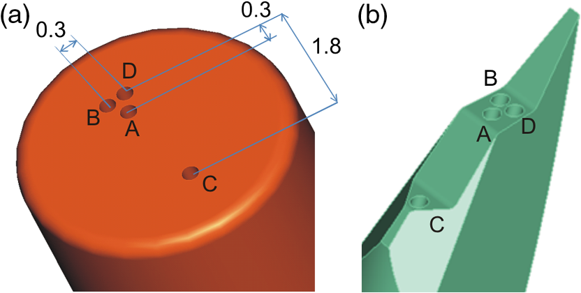

During each measurement, three spectra are acquired: a fluorescence spectrum and diffuse reflectance spectra at the short fiber distance ( $δ = 0.3 mm$ ) and the long fiber distance ( $δ = 1.8 mm$ ). From the DRS measurement the absorption and the reduced scattering coefficients are determined for all wavelengths involved. This is done by fitting the spectra with the diffusion theory model of Refs. 13 and 19. The absorption coefficients $μ_{a m}$ and $μ_{a x}$ are determined from the extinction spectra of the individual chromophores using the concentrations as fitting parameters, while the reduced scattering coefficients $μ_{s x}^{'}$ and $μ_{s m}^{'}$ are approximated by a superposition of two exponential functions (one for Mie and one for Rayleigh scattering). A Levenberg-Marquardt nonlinear fitting algorithm is used to optimize the chromophores concentrations and scattering parameter. The algorithm is described and validated in detail in Refs. 18 and 20. The algorithm generally yields very good agreement between measured and fitted DRS spectra. A drawback is that the model requires that the extinction spectra of all absorbers are known. Also, the algorithm becomes less reliable for short fiber distances ( $ρ < 1 mm$ ) because the diffusion approximation breaks down. As a result, one typically obtains a different set of $μ_{s}^{'}$ and $μ_{a}$ from the short distance (SD) DRS measurement than from the long distance (LD) with the long distance set being more trustworthy.

To determine the intrinsic fluorescence according to the MüllerZhang method, first the measured short distance DRS spectrum is fitted by the diffusion theory model as described above. From this fit the albedo $a_{m}$ can be determined. Furthermore, we can deduce the scattering in absence of absorption by setting the absorption coefficient from this fit equal to zero yielding $R_{0}$ . In the MüllerZhang method, the probe-specific parameters $S$ and $l$ are determined from measurements on known samples. From this $S$ we can then determine $β$ and subsequently $ε$ . Inserting $S$ , $l, ε$ , and the measured $R$ and $F_{x m}$ in Eq. (10) yield the intrinsic fluorescence. In the MPM method, the parameters $S$ and $l$ are not a priori known. Here, we determine $κ$ using the relation $κ = R_{0} (e^{β} - 1)$ . Inserting $a_{m}$ , $R_{0}$ , and $κ$ in Eq. (6) and using for $R$ the measured short distance DRS spectrum we can deduce the parameter $β$ and thus the parameter $ϵ = (e^{β} - 1)$ . From Eq. (10) we can then deduce the intrinsic fluorescence from the measured fluorescence $F_{x m}$ apart from a scaling factor.

To determine the intrinsic fluorescence with the Monte Carlo look-up table (MCLUT) method, Eq. (15) is employed to calculate $ϕ_{x m}^{eff}$ , making use of the calculated previously look-up table for $k_{x m}$ . Then, Eq. (12) is used to determine the intrinsic fluorescence $f_{x m}$ , as defined above. This can be done with the $μ_{s}^{'} - μ_{a}$ -set from the short or the long distance DRS measurement, resulting in two different intrinsic fluorescence spectra, which we call short MCLUT and long MCLUT.

If the intrinsic fluorescence spectra $η_{i}$ of the individual fluorophores are known, then the (relative) concentrations $c_{i}$ of the fluorophores can be determined by fitting $f_{x m}$ according to Eq. (3) with the $c_{i}$ as fit parameters. We are only interested in relative concentrations, so we set $ε$ and $ϕ_{x m}$ to 1 as scaling factors.

2.5.

Tissue Phantom Preparation

To validate the MCLUT method, phantoms with a single fluorophore are made by diluting latex balls (scatterer, diameter $diameter \approx 1 μ m$ , Duke Scientific), red tissue marking dye (absorber, #63020-RD, Electron Microscopy Sciences), and a Lucifer Yellow preparation (fluorophore) in distilled water. These phantoms were also used to determine the constants $S$ and $l$ for the flat-head-probe according to Ref. 5.

To compare the different techniques of reconstructing the intrinsic fluorescence spectra in a quantitative way, a series of phantoms are prepared. They contain a mixture of two different fluorophores in various concentration ratios and an absorber in various concentrations. The diffuse reflectance and fluorescence spectra of the phantoms are measured and the intrinsic fluorescence spectrum of each phantom is recovered using all three techniques. From the recovered intrinsic fluorescence spectra the ratio of the two fluorophores in the phantom is determined. The deviation of the fluorophore ratio determined, thus from the true fluorophore ratio is taken as a measure for the quality of the recovery algorithm.

Nine phantoms were made, called N1 to N9. All phantoms contain the same amount of scatterers. The scatterers are Polybead® polystyrene microspheres from Polysciences, Inc. with a diameter of $1.025 \pm 0.01 μ m$ . The initial suspension was diluted in demiwater to a polystyrene concentration of 2.4 V%. The absorbers used are a mixture of Amaranth and Tartrazine from SigmaAldrich. Amaranth and Tartrazine are both red food dyes with a high stability against photo-bleaching. Using a mixture creates a more characteristic absorption spectra than a single absorber. The extinction spectrum of the mixture was measured and it showed two distinct absorption maxima at 434 and at 522 nm. Phantoms N1, N2, and N3 are prepared with 5 V% of the absorber mix, phantoms N4, N5, and N6 with 1.25 V%, and phantoms N7 and N8 with 0.5 V%. Phantom N9 does not contain any absorber and is used as a reference.

The fluorophores used are preparations of Stilben-3 and brilliant Sulfaflavin in demiwater. Three different combinations of the two fluorophores were used. Both fluorophores have broad fluorescence peaks with a maximum around 425 nm (Stilben-3) and 525 nm (brilliant Sulfaflavin). These two peaks will typically still be visible in the intrinsic fluorescence spectra of a mixture, with the relative height of the peaks depending on the Stilben3/Sulfaflavin ratio. Phantoms N1, N4, and N7 were prepared with an (arbitrarily scaled) Stilben3/Sulfaflavin ratio of 1; N2, N5, and N8 with a Stilben3/Sulfaflavin ratio of 2.75; and N3 and N6 with Stilben3/Sulfaflavin ratio of 0.26. These ratios were determined by measuring the fluorescence spectra of the various mixtures and then fitting the spectra of the individual fluorophores. The intrinsic fluorescence spectrum of all fluorophore preparations are measured on the undiluted preparation without any additional absorbers or scatterer present.

2.6.

Biological Tissue Measurements

To determine the applicability of the MPM and MCLUT techniques to biological tissue, we also measured various ex vivo human tissue samples. These measurements were conducted at The Netherlands Cancer Institute (NKI-AVL) under approval of the internal review board. Tissue samples from lung, liver, breast, and cervix are obtained from patients undergoing a surgical tumor resection. The freshly excised tissues are grossly inspected by a pathologist prior to our measurements. A different optical probe is used with a sharp step-like tip [see Fig. 1(b)] that can penetrate the tissue and measure inside the tissue volume. The measurements on cervical tissue are done on the surface of the ectocervix with the flat-head probe. The analysis is done as described above for the phantoms. No good values for the constants $l$ and $S$ are available for the step probe so the original MüllerZhang method is not used for the biological samples.

3. Results

3.1.

Examples of Look-Up Tables

Figure 2 shows two typical examples of the look-up table $k_{x m}$ calculated with our Monte Carlo routine. The images only show a two-dimensional subset where the values at the excitation wavelength are kept fixed at $μ_{s x}^{'} = 1.25 {mm}^{- 1}$ and $μ_{a x} = 2.0 {mm}^{- 1}$ in (a) and at $μ_{s x}^{'} = 5.0 {mm}^{- 1}$ and $μ_{a x} = 1.5 {mm}^{- 1}$ in (b) both for a source-detector fiber distance $ρ = 0.3 mm$ . As one would expect, the correction factor $k_{x m}$ decreases for increasing $μ_{a m}$ , i.e., the measured fluorescence intensity decreases with increased absorption at the emission wavelength. The influence of $μ_{s m}^{'}$ is more complicated. For low values of $μ_{a m}^{'}$ there exists a maximum $k_{x m}$ , i.e., an increase of the scattering coefficient $μ_{s m}^{'}$ increases the measured fluorescence intensity until a maximum is reached after which a further increase in $μ_{s m}^{'}$ results in a sharp drop. The maximum grows less pronounced and finally disappears when the absorption coefficient $μ_{a m}^{'}$ increases further.

Fig. 2

Example of two $k_{x m} (μ_{s x}, μ_{a x}^{'}, μ_{s m}, μ_{a m}^{'})$ look-up tables. The full look-up table is four-dimensional; the image shows only the $μ_{s m}^{'} - μ_{a m}$ curves for two different fixed $μ_{s x}^{'} - μ_{a x}$ combinations: (a) $μ_{s x}^{'} = 1.25 {mm}^{- 1}$ , $μ_{a x} = 2 {mm}^{- 1}$ and (b) $μ_{s x}^{'} = 5 {mm}^{- 1}$ , $μ_{a x} = 1.5 {mm}^{- 1}$ , $ρ = 0.3 mm$ .

Figure 3(a) shows the dependence of $k_{x m}$ when scattering and absorption properties are varied at the excitation wavelength for fixed $μ_{s m}^{'} = 10 {mm}^{- 1}$ , $μ_{a m} = 1 {mm}^{- 1}$ . The correction factor $k_{x m}$ shows variations of the same order of magnitude as when varying the parameters at the detection wavelength.

Fig. 3

(a) Example of a $k_{x m}$ look-up table for a fixed $μ_{s m}^{'} - μ_{a m}$ combination: $μ_{s m}^{'} = 10 {mm}^{- 1}$ , $μ_{a m} = 1 {mm}^{- 1}$ . (b) Calculated correction curves for identical ( $μ_{s m}^{'}$ , $μ_{a m}$ ) spectra but different $μ_{s x}^{'}$ , and $μ_{a x}$ combinations. The curves were calculated for $μ_{s m}^{'} = 1 {mm}^{- 1}$ and for the $μ_{a m}$ -spectrum determined by a blood concentration of $0.75 mg / ml$ oxyhemoglobin.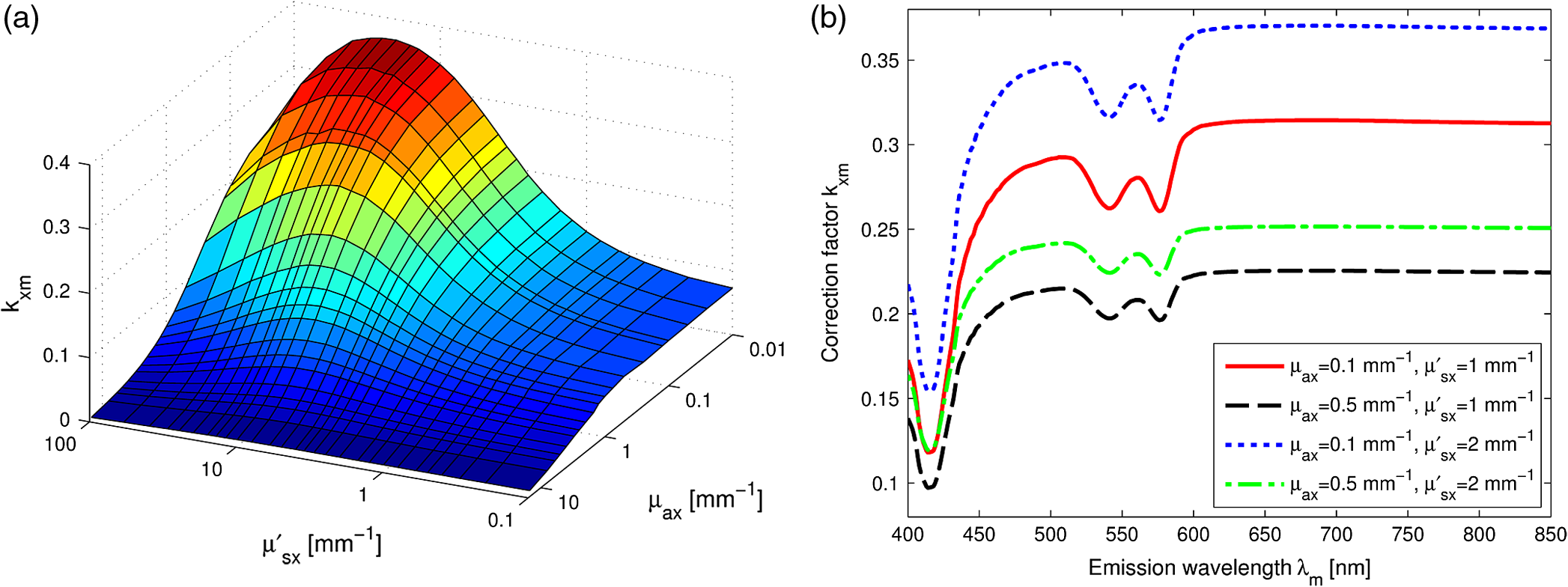

For monochromatic excitation, there is only one value for $μ_{s x}^{'}$ and $μ_{a x}$ but a different ( $μ_{a m}^{'}$ , $μ_{a m}$ ) duplet for every measured emission wavelength. Using those as input for the look-up table yields a correction factor spectrum $k_{x m} (λ_{m})$ . Figure 3(b) depicts four such spectra, using the same ( $μ_{s m}^{'}$ , $μ_{a m}$ ) spectrum but with moderate differences in the $μ_{s x}^{'}$ , and $μ_{a x}$ values. These differences cause significant deviations in the absolute values of the correction factor but also noticeable changes in the shape of the curves.

3.2.

Recovery of the Intrinsic Fluorescence Spectrum Using the Monte Carlo Look-Up Table

This section describes the recovery of the intrinsic fluorescence spectrum using the MCLUT method. As an example, we consider the phantom with one absorber, one fluorophore, and one type of scatters (see Sec. 2.5).

Figure 4 shows the DRS and fluorescence spectra measured on the single fluorophore phantom. The red paint has absorption peaks at 528 and 571 nm, which are clearly visible in the DRS spectrum and the latter also in the fluorescence spectrum. The absorption clearly has a major influence on the measured fluorescence spectra, which looks very different from the real intrinsic fluorescence of the fluorophore [Fig. 4(b)].

Fig. 4

Plot of (a) the measured reflectance spectrum and the calculated correction factor $k_{x m}$ and (b) the measured fluorescence spectrum and the recovered fluorescence spectra compared to the measured intrinsic fluorescence spectrum of the pure fluorophore preparation. All graphs are scaled to facilitate comparison.

From the $μ_{s x}^{'}$ , $μ_{a x}^{'}$ , $μ_{s m}$ , and $μ_{a m}$ from the short distance measurement the correction factor $k_{x m}$ is determined by interpolation from the look-up table [Fig. 4(a)]. It is obvious that $k_{x m}$ has similar features as the measured reflectance spectrum. Figure 4(b) shows the recovered intrinsic fluorescence spectrum using the MCLUT technique. Good agreement between the recovered intrinsic fluorescence spectra and the fluorescence spectra measured on the pure fluorophore preparation is obtained.

3.3.

Comparison of Different Methods for Obtaining the Intrinsic Fluorescence on Phantoms

In this section, the recovery of the intrinsic fluorescence of the nine samples (N1 to N9) will be discussed. All samples are measured with the probe and setup described in Sec. 2.4, with DRS measurements being taken at both the short and the long distance. Figure 5 shows the DRS measurements and the resulting fits for two of the phantoms. Agreement between the measurement and the fits is limited by the uniform size of the scatterers, which causes ripples in the $μ_{s m}^{'}$ -spectra that cannot be reproduced by the exponential function used. Figure 6 depicts for the same two phantoms the measured fluorescence curves, the intrinsic fluorescence curve of the fluorophore mixture, and the intrinsic fluorescence curves recovered with the MüllerZhang, MPM, and MCLUT. The Monte Carlo look-up table method is used with both the short and the long DRS measurement.

Fig. 5

DRS measurement curves (solid lines) with fitted curve (dotted lines) at short (black) and long distances (red) for the phantoms (a) N1 and (b) N6. The long-distance curves were multiplied with 7 to enhance the visibility.

Fig. 6

The directly measured and the recovered intrinsic fluorescence spectrum of phantoms (a) N1 and (b) N6. The graphs are scaled so that the integral under the curve is 1.

Although not shown in this paper, the recovered intrinsic fluorescence of the other phantoms exhibit similar results: the strong absorption dips are removed from the fluorescence spectra for all the methods used. However, the relative heights of the two fluorescence peaks are rarely recovered correctly. Furthermore, the fluorescence intensity $> 600 nm$ is decreasing slower than observed in the real intrinsic fluorescence regardless of the method used. It is not clear whether this “tail” is caused by the algorithms or whether it is due to actual additional fluorescence (e.g., by the fiber probe or by the polystyrene microspheres).

To derive a measure for the quality of the fit, the reconstructed fluorescence curve is fitted as a superposition of the individual intrinsic fluorescence curves of Stilben 3 and brilliant Sulfaflavin. This fitting was done in the wavelength range from 405 to 575 nm to limit the influence of the low intensity, long wavelength “tail” on the result. From the fitting results the Stilben3/Sulfaflavin ratio is calculated. Table 1 lists the deviations (in %) from the expected Stilben3/Sulfaflavin ratio for each sample for the various methods used. The last two rows in Table 1 give the mean and the standard deviation for each technique.

Table 1

Deviation of the recovered fluorophore ratios (Stilben3/Sulfaflavin) from the expected ratio expressed in percentage (%) for eight phantom samples. The row labeled Σ2 gives the sum of the squared deviations for each method. The average deviation (average) over the eight samples and the standard deviation (STDEV) are given as well.

		Method
		MPM	MüllerZhang	MCLUT (short)	MCLUT (long)
Sample	N1	$- 14 %$	$- 15 %$	0%	$- 13 %$
	N2	$- 33 %$	$- 36 %$	$- 9 %$	$- 31 %$
	N3	33%	31%	48%	30%
	N4	$- 3 %$	$- 1 %$	$- 2 %$	$- 9 %$
	N5	$- 16 %$	$- 13 %$	$- 16 %$	$- 26 %$
	N6	39%	41%	39%	32%
	N7	14%	18%	$- 11 %$	$- 13 %$
	N8	16%	27%	$- 26 %$	$- 28 %$
$Σ^{2}$		0.46	0.53	0.49	0.47
Mean		5%	6%	3%	$- 7 %$
STDEV		24%	25%	25%	23%

3.4.

Recovering the Intrinsic Fluorescence of Biological Tissue in Practice

In this section, different intrinsic fluorescence recovery methods shall be compared when applied to human breast, lung, liver, and cervix tissue samples. Typical examples of the DRS and fluorescence spectra obtained from these human tissue samples are shown in Fig. 7. To retrieve the scattering and absorption from the DRS spectrum, we apply the fitting as described above taking the chromophores hemoglobin, deoxyhemoglobin, water, lipid, beta-carotene, collagen, and bile (for liver samples) into account. In Fig. 7(a), 7(c), and 7(g) the double dip structure due to oxyhemoglobin near 550 nm is clearly visible and fitted well in these three cases. In Fig. 7(e), i.e., liver tissue, the double dip is less prominent and the blood is more deoxygenated. When we compare the recovered intrinsic fluorescence according to the MPM method with the MCLUT method, we observe that the intrinsic fluorescence reconstruction of the MPM and the short distance MCLUT methods are similar. In comparison, the long distance MCLUT methods seems to result in an “undercorrection,” meaning that the long distance MCLUT result is closer to the original measured spectra than those of the other methods. Apart from lung and liver where the absorption due to blood is large, the three models predict similar results for the recovered intrinsic fluorescence.

Fig. 7

Short- and long-distance DRS measurements and the fit result for (a) breast, (c) lung, (e) liver, and (g) cervix human tissue are given. In (b), (d), (f), and (h), the corresponding fluorescence spectrum and the recovered spectrum according to the MPM, MCLUT SD, and MCLUT LD are presented, respectively.

4. Discussion

This paper reveals different ways to recover the intrinsic fluorescence spectrum from measured spectra of the fluorescence and the diffuse reflectance in turbid media. The MCLUT technique is, as far as the authors know, the first time that a look-up table has been used for this purpose.

The shape of the look-up table calculated by the Monte Carlo routine is complex but plausible: with increasing absorption, both at the excitation and the emission wavelength, the measured fluorescence decreases [Figs. 2 and 3(a)]. The influence of scattering is more complicated. The scattering coefficient at the emission wavelengths inversely correlates with the maximum distance from the fluorophore that, on average, the emitted photon will reach on its random walk through the tissue. Therefore, increasing $μ_{s m}^{'}$ at first raises the measured fluorescence as the photon density at the collection fiber increases but then decreases because most photons cannot reach the collection fiber anymore. This explains the maximum in Fig. 2(a) and 2(b). Varying the scattering at the excitation wavelength also produces a maximum in the fluorescence intensity for medium $μ_{s x}^{'}$ . For low scattering, the excitation photons can enter deep into the tissue before being absorbed by a fluorophore, resulting in very few fluorescent photons exiting the tissue. For large $μ_{s x}^{'}$ , the excitation photons will be absorbed very close to the delivery fiber and many photons will be scattered out of the tissue without being absorbed. Therefore, maximum collection of fluorescent photons occurs for medium scattering at the excitation wavelength.

This complex dependency of $k_{x m}$ on the optical properties at both the emission and the excitation wavelength justifies using a four-dimensional look-up table. In particular, the influence of $μ_{s x}^{'}$ and $μ_{a x}$ cannot be described by a simple scaling parameter. This is demonstrated in the examples in Fig. 3(b) where a comparison of, e.g., the solid red curve with the dash-dotted green curve shows that the shape of a correction spectrum can vary significantly if the optical properties at the excitation wavelengths change. This four-dimensionality is an important difference between the look-up table methods and the photon-migration based methods, since the latter does not consider the optical properties at the excitation wavelength except for using $μ_{s x}$ as a scaling factor.

On the tissue phantoms, the various techniques to reconstruct the intrinsic fluorescence all perform reasonably well. The strong absorption dips are filtered out regardless of the method used. However, the various methods produce subtly different shapes for the intrinsic fluorescence spectra that affect the determined relative fluorophore concentrations. These determined ratios of fluorophore concentrations were used as a measure of the goodness of intrinsic fluorescence reconstruction.

Table 1 shows that none of the methods works best for all samples. To get a figure of merit for the overall quality of each technique, the relative deviations are squared and summed up (see the row labeled $Σ^{2}$ in Table 1). By this measure, the MPM and the MCLUT methods using the data from the long distance measurement yield the best results. The MCLUT method making use of the short distance diffuse reflectance measurement and the MüllerZhang method perform somewhat less well but the differences are marginal.

A common issue is caused by the fact that the source-detector fiber distance is of the same order of magnitude as the typical scattering length. This means that the light transport in tissue does not comply with the criteria necessary for the diffusion approximation to hold. In all the methods investigated in this paper, the step to retrieve the scattering and absorption parameter rely on this diffusion theory. In the MüllerZhang method and the MPM this is partly solved by using only the scattering information (i.e., the function $R_{0}$ ) determined by this diffusion theory fit while the absorption is only taken into account by using the separately measured diffuse reflectance spectrum $R_{m}$ . For the MCLUT methods, however, this is a serious issue when the short distance DRS measurement is used. The MCLUT using the long distance DRS measurement is affected least. The problem with the diffusion approximation for short distances therefore explains why the long MCLUT works slightly better than the short MCLUT for the phantom measurements. These fitting errors might be lessened by employing, instead of the diffusion approximation based fitting of the DRS spectrum, an inverse Monte Carlo based fitting of the DRS spectrum.

The slightly improved performance of the MPM compared to the original MüllerZhang method might be explained by the additional freedom in the MPM method, where the parameters $l$ and $S$ are determined in each fit separately, compared to the MüllerZhang method, where they are determined once based on various test phantoms.

Care must be taken with the ranking of the various methods to recover the intrinsic fluorescence used in the report. As measurements were only done on a small number of similar phantoms, there remains a large margin for statistical and systematic errors. For example, it appears as if all reconstruction methods produce increasing errors for phantoms with decreasing Stilben3/Sulfaflavin ratios, but it is unclear whether it is a real effect or a statistical artifact and, if it is a real effect, whether it is caused by our special choice of tissue phantom. Further investigation on this point is required. Also, the method chosen to compare the various techniques is rather arbitrary, even though recovering the intrinsic fluorescence spectra and determining the fluorophore concentrations from it is of large practical relevance. Still, we believe that the phantom measurements give a good first impression of the performance one can expect from the various intrinsic fluorescence recovery methods. To the best of our knowledge, this is the first attempt of a quantitative comparison of different techniques. In general, we can conclude that the various methods are able to reconstruct the intrinsic fluorescence but the error in the reconstruction can lead to errors in relative concentration on average of up to 25% (i.e., one standard deviation) as found in our examples.

From the examples presented on human breast, lung, liver, and cervix tissue we observe that the MPM and short distance MCLUT methods produce similar results for the recovered intrinsic fluorescence. For breast and cervix tissue these agree with the results from the long distance MCLUT method. Although no benchmark with the real intrinsic fluorescence can be made, these results are promising since the results are obtained with two highly independent reconstruction methods. When we compare the DRS spectra measured for this human tissue with the phantom studied, we observe that the amount of absorption and scattering present is of the same ballpark figure. Therefore, we expect that the recovery of the intrinsic fluorescence also has an accuracy similar to that of the recovery of the tissue phantoms. However, there may be additional unknown chromophores present in the biological tissues which may cause additional errors in the DRS fit and decrease the overall accuracy.

The long distance MCLUT method produced rather different reconstructions in tissues with strong absorption bands [Fig. 7(c) and 7(e)]. One also sees that traces of the blood absorption bands remain in the recovered intrinsic fluorescence spectra [Fig. 7(d) and 7(f)]. We attribute this to a low fidelity in the reconstruction of the $μ_{a}$ and $μ_{s}^{'}$ values due to strong tissue inhomogeneities, high absorption, and a complicated probe geometry. In order for the MCLUT method to work, the optical properties in the volumes from the fluorescence and the DRS measurements have to be similar. This was the case for the phantoms, but biological tissues are much less homogenous. This is mainly an issue when using the long distance DRS measurement since it measures a much larger volume with less overlap with fluorescence volume. Also, for samples with high blood content (liver, lung), the long distance of the probe used was too long, resulting in excessive absorption. In Fig. 7(c) and 7(d), the intensity of the long distance DRS measurements in the absorption bands is practically zero. With the most characteristic part of the spectrum gone, fitting errors increase and the long-distance DRS fit becomes imprecise. This may attribute to the underfitting seen in Fig. 7(b) and 7(c) in the short wavelength regions. Last but not least, the complicated geometry of the fiber optical probe which was necessary to penetrate into tissue [Fig. 1(b)] might have added additional distortions to the long-distance DRS spectrum (even though the fiber distances are the same for both types of probe). For these reasons, we believe that for liver and long tissues the long-distance MCLUT results are less accurate than the results from the short-distance MCLUT and from MPM.

In general, the MCLUT method depends more on the quality of the DRS fit than the MPM method. This is because $μ_{a}$ and $μ_{s}^{'}$ are more sensitive to fitting errors than $R_{0}$ . This reduced robustness may offset the advantage of not having to measure fluorescence and DRS in the same geometry. Since the computational effort is preloaded in calculating the look-up table, the recovery itself is fast and computationally cheap. Overall, the results show that it is possible to accurately recover the intrinsic fluorescence spectrum from a short-distance fluorescence measurement using the MCLUT method with only a long-distance DRS measurement. Results are best when the sample is homogenous on the scale of the long distance and has no absorption bands strong enough to introduce errors in the DRS fit.

5. Summary and Conclusions

A new method based on Monte Carlo look-up-tables to recover intrinsic fluorescence from measured fluorescence on turbid media has been presented. This new method requires an additional diffuse reflectance measurement taken at the same location as the fluorescence measurement but not necessarily with the same probe geometry. The method has been validated on various phantoms with known intrinsic fluorescence. The MCLUT was also benchmarked against the photon-migration method for intrinsic fluorescence recovery developed by Müller et al. and Zhang et al. (MüllerZhang method) and with a slightly modified photon-migration method that does not need prior knowledge of optical probe specific parameters. These methods require a diffuse reflectance spectrum measurement taken at the same location and with the same optical probe geometry as the fluorescence measurement. The MCLUT showed similar reconstruction accuracy as the methods based on the photon-migration method. Furthermore, also the MCLUT with different probe geometry for the DRS measurement resulted in similar intrinsic fluorescence reconstruction as the photon-migration method as long as the source-detector fiber distance is chosen such that the DRS spectrum in the relevant wavelength region is well detectable while, furthermore, the fiber distance is smaller than the average scale of the tissue inhomogenities. The modified photon-migration based method proposed in this paper resulted in a slightly improved result than found with the original MüllerZhang method.

In the current MCLUT method, the absorption and scattering parameters are determined from the DRS measurement by employing a diffusion theory model based fitting. The MCLUT method is therefore sensitive for errors in both absorption and scattering coefficient. The photon-migration based model uses only the scattering coefficient from this fitting step, making this method less sensitive for fitting errors than the MCLUT in the current form. In general, we can conclude that the MCLUT is a promising technique to recover the intrinsic fluorescence of biological tissues. It combines more flexibility in the probe design and fast reconstruction times with similar accuracy in reconstruction of the intrinsic fluorescence as found in the photon-migration based reconstruction methods.

Acknowledgments

We thank Prof. S. L. Jacques (Oregon Medical Laser Center) for providing the mfluor.c code to benchmark our Monte Carlo program code. Prof. Theo Ruers (Netherlands Cancer Institute) is acknowledged for enabling the measurements on the human tissue samples. We thank Rami Nachabé and Arnold van Keersop for their support in writing the MPM code, Walter Bierhoff for providing the optical probes, and Jeroen Horikx for providing the optical console.

Appendices

Appendix:

Validation of the Monte Carlo Routines

To validate our Monte Carlo program, we benchmarked our Monte Carlo routines with existing peer-reviewed Monte Carlo routines. The basic Monte Carlo routine and the calculation of $A (r, z)$ were validated by comparing selected outputs with results produced by the program MCML by Wang et al.¹⁴ Both programs were in excellent agreement.

To validate the full fluorescence routine (called fluostitch.m), the program mcfluor.c from Prof. S. L. Jacques was employed.¹⁷ Figure 8(a) shows the distribution of the fluorescence intensity $F (ρ)$ calculated both with mcfluor.c and with fluostitch.m for three different tissue parameter sets. To obtain the same accuracy required longer computation times for mclfuor.c program than our new code fluostitch.c. Figure 8(b) shows the results of another comparison between the two programs. Instead of showing the whole spectrum $F (ρ)$ , only the values at two distances are compared. The tissue properties at the excitation wavelength are kept constant but are varied at the emission wavelength. The graph shows again, a good agreement. The deviations are of the same order of magnitude as the noise present in the data points.

Fig. 8

Comparison of our fluorescence Monte Carlo routine fluostitch.m with the mcfluor.c program. (a) Distribution of fluorescence intensity versus source-detector fiber distance $ρ$ for three parameter sets each. Both types of curves are scaled so that for the parameter set 2 the fluorescence equals 1 for $ρ = 0.2 mm$ . Set 1: $μ_{s x}^{'} = 0.5 {mm}^{- 1}$ , $μ_{a x} = 1 {mm}^{- 1}$ , $μ_{s m}^{'} = 2 {mm}^{- 1}$ , $μ_{a m} = 0.5 {mm}^{- 1}$ ; Set 2: $μ_{s x}^{'} = 5 {mm}^{- 1}$ , $μ_{a x} = 0.25 {mm}^{- 1}$ , $μ_{s m}^{'} = 3 {mm}^{- 1}$ , $μ_{a m} = 0.5 {mm}^{- 1}$ ; Set 3: $μ_{s x} = 2 {mm}^{- 1}$ , $μ_{a x} = 1 {mm}^{- 1}$ , $μ_{s m}^{'} = 1 {mm}^{- 1}$ , $μ_{a m} = 0.25 {mm}^{- 1}$ . (b) Fluorescence intensity for different parameter sets calculated with fluostitch.m and mcfluor.c for two different source-detector fiber distances, $ρ = 0.5 mm$ and $ρ = 1 mm$ . The excitation properties were identical in all cases, $μ_{s x} = 10 {mm}^{- 1}$ , $μ_{a x} = 1 {mm}^{- 1}$ , while the emission properties were $μ_{s m} = 20$ , 10, and $5 {mm}^{- 1}$ for 1, 2, and 3, respectively, and, $μ_{a m} = 0.5$ , 1, and $0.25 {mm}^{- 1}$ for A, B, and C, respectively. Both types are scaled so that for the parameter set 1A the fluorescence equals 1 for 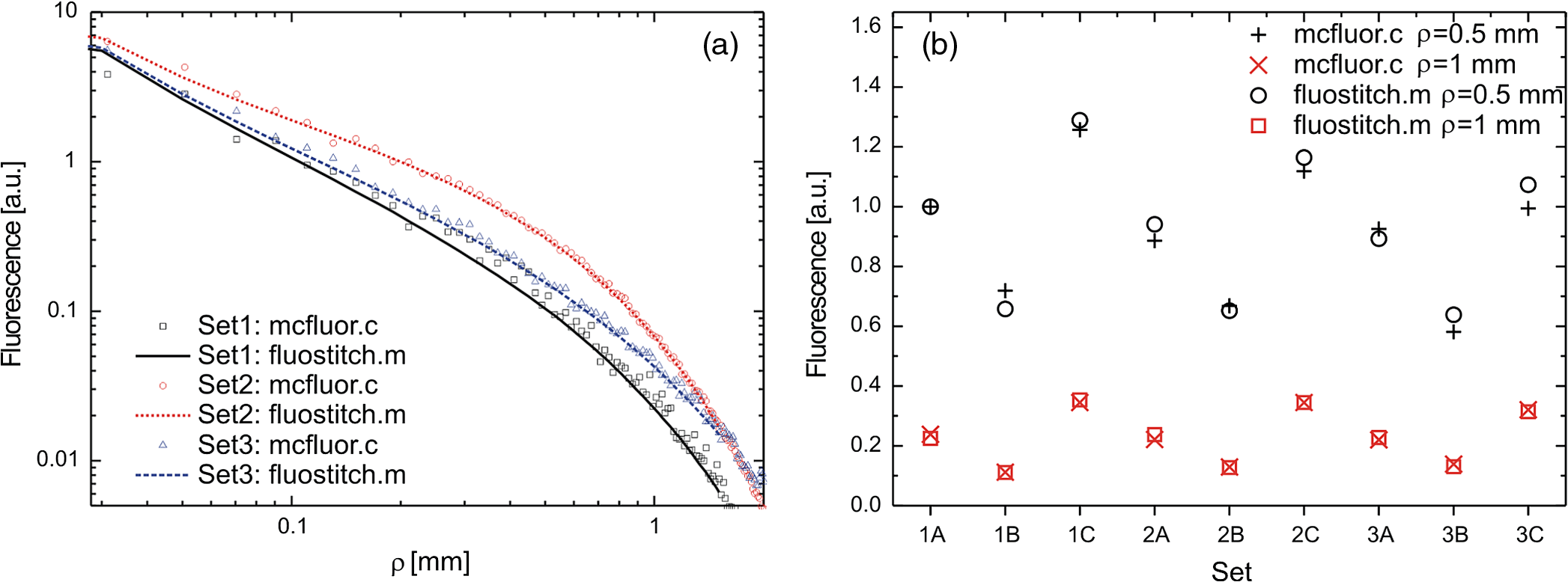$ρ = 0.5 mm$ .

References

1.

R. Richards-KortumE. Sevick-Muraca, “Quantitative spectroscopy for tissue diagnosis,” Annu. Rev. Phys. Chem., 47 (1), 555 –606 (1996). http://dx.doi.org/10.1146/annurev.physchem.47.1.555 ARPLAP 0066-426X Google Scholar

2.

G. A. WagnieresW. M. StarB. C. Wilson, “ln vivo fluorescence spectroscopy and imaging for oncological applications,” Photochem. Photobiol., 68 (5), 603 –632 (1998). http://dx.doi.org/10.1111/php.1998.68.issue-5 PHCBAP 0031-8655 Google Scholar

3.

R. S. BradleyM. S. Thorniley, “A review of attenuation correction techniques for tissue fluorescence,” J. R. Soc. Interface, 3 (6), 1 –13 (2006). http://dx.doi.org/10.1098/rsif.2005.0066 1742-5689 Google Scholar

4.

Q. Zhanget al., “Turbidity-free fluorescence spectroscopy of biological tissue,” Opt. Lett., 25 (19), 1451 –1453 (2000). http://dx.doi.org/10.1364/OL.25.001451 OPLEDP 0146-9592 Google Scholar

5.

M. G. Mülleret al., “Intrinsic fluorescence spectroscopy in a turbid media—disentangling effects of scattering and absorption,” Appl. Opt., 40 (25), 4633 –4646 (2001). http://dx.doi.org/10.1364/AO.40.004633 APOPAI 0003-6935 Google Scholar

6.

T. J. FarrellM. S. PattersonB. Wilson, “A diffusion theory model of spatially resolved, steady-state diffuse reflectance for the non-invasive determination of tissue optical properties,” Med. Phys., 19 (4), 879 –888 (1992). http://dx.doi.org/10.1118/1.596777 MPHYA6 0094-2405 Google Scholar

7.

M. SinaasappelM. H. J. C. Sterenborg, “Quantification of the hematoporphyrin derivative by fluorescence measurement using dual-wavelength excitation and dual-wavelength detection,” Appl. Opt., 32 (4), 541 –548 (1993). http://dx.doi.org/10.1364/AO.32.000541 APOPAI 0003-6935 Google Scholar

8.

G. M. PalmerN. Ramanujam, “Monte-Carlo-based model for the extraction of intrinsic fluorescence from turbid media,” J. Biomed. Opt., 13 (2), 024017 (2008). http://dx.doi.org/10.1117/1.2907161 JBOPFO 1083-3668 Google Scholar

9.

L.-H. WangH. Wu, Biomedical Optics—Principles and Imaging, Wiley-Interscience, Hoboken, New Jersey (2007). Google Scholar

10.

J. MobleyT. Vo-Din, “Optical properties of tissue,” Biomedical Photonics Handbook, CRC Press LLC, Boca Raton (2003). Google Scholar

11.

J. WuM. S. FeldR. P. Rava, “Analytical model for extracting intrinsic fluorescence in turbid media,” Appl. Opt., 32 (19), 3585 –3595 (1993). http://dx.doi.org/10.1364/AO.32.003585 APOPAI 0003-6935 Google Scholar

12.

J. Swartlinget al., “Accelerated Monte Carlo models to simulate fluorescence spectra from layered tissue,” J. Opt. Soc. Am. A, 20 (4), 714 –727 (2003). http://dx.doi.org/10.1364/JOSAA.20.000714 JOAOD6 0740-3232 Google Scholar

13.

N. RajaramT. H. NguyenJ. W. Tunnell, “Lookup table based inverse model for determining optical properties of turbid media,” J. Biomed. Opt., 13 (5), 050501 (2008). http://dx.doi.org/10.1117/1.2981797 JBOPFO 1083-3668 Google Scholar

14.

L.-H. WangS. L. JacquesL.-Q. Zheng, “MCML—Monte Carlo modeling of photon transport in multi-layered tissues,” Comput. Methods Programs Biomed., 47 (2), 131 –146 (1995). http://dx.doi.org/10.1016/0169-2607(95)01640-F CMPBEK 0169-2607 Google Scholar

15.

A. J. Welchet al., “Propagation of fluorescent light,” Laser. Surg. Med., 21 (2), 166 –178 (1997). http://dx.doi.org/10.1002/(ISSN)1096-9101 LSMEDI 0196-8092 Google Scholar

16.

D. E. Hydeet al., “A diffusion theory model of spatially resolved fluorescence from depth-dependent fluorophore concentrations,” Phys. Med. Biol., 46 (2), 369 –383 (2001). http://dx.doi.org/10.1088/0031-9155/46/2/307 PHMBA7 0031-9155 Google Scholar

17.

S. L. Jacques, “Monte Carlo simulations of fluorescence in turbid media,” Handbook of Biomedical Fluorescence, Marcel-Dekker, New York (2003). Google Scholar

18.

R. Nachabéet al., “Estimation of lipid and water concentrations in scattering media with diffuse optical spectroscopy from 900 to 1600 nm,” J. Biomed. Opt., 15 (3), 037015 (2010). http://dx.doi.org/10.1117/1.3454392 JBOPFO 1083-3668 Google Scholar

19.

G. Zonioset al., “Diffuse reflectance spectroscopy of human adenomatous colon polyps in vivo,” Appl. Opt., 38 (31), 6628 –6637 (1999). http://dx.doi.org/10.1364/AO.38.006628 APOPAI 0003-6935 Google Scholar

20.

R. Nachabéet al., “Estimation of biological chromophores using diffuse optical spectroscopy: benefit of extending the UV-VIS wavelength range to include 1000 to 1600 nm,” Biomed. Opt. Express, 1 (5), 1432 –1442 (2010). http://dx.doi.org/10.1364/BOE.1.001432 OPEXFF 1094-4087 Google Scholar

CC BY: © The Authors. Published by SPIE under a Creative Commons Attribution 4.0 Unported License. Distribution or reproduction of this work in whole or in part requires full attribution of the original publication, including its DOI.

Citation Download Citation

Manfred Muller and Benno H. W. Hendriks "Recovering intrinsic fluorescence by Monte Carlo modeling," Journal of Biomedical Optics 18(2), 027009 (11 February 2013). https://doi.org/10.1117/1.JBO.18.2.027009

Published: 11 February 2013

Access the abstract

JOURNAL ARTICLE
14 PAGES

DOWNLOAD PAPER SAVE TO MY LIBRARY

GET CITATION

CITATIONS

Cited by 16 scholarly publications and 17 patents.

Explore citations on Lens.org

KEYWORDS

Luminescence

Tissues

Absorption

Monte Carlo methods

Scattering

Distance measurement

Diffuse reflectance spectroscopy

1.

Introduction

2.

Materials and Methods