|
|
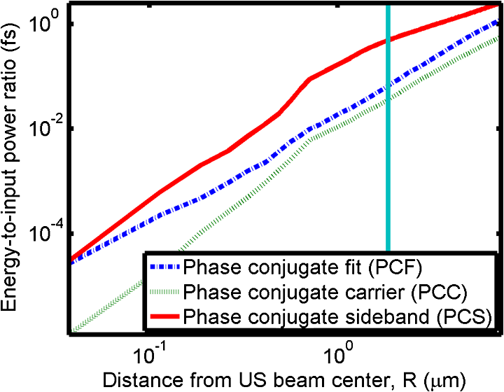
1.IntroductionOptical interrogation of tissue provides noninvasive imaging, excellent resolution, and deep penetration. However, strong scattering distorts wavefronts as they pass through tissue and does not allow these three benefits to be achieved simultaneously. Optical wave distortions are routinely corrected in astronomy with adaptive optics.1,2 The atmosphere introduces aberrations in the wavefront of terrestrially measured starlight. In the absence of atmospheric turbulence, the wavefront measured by a telescope would appear to be planar because the telescope is in the far field of the “guidestar.” Any variation from a plane wavefront caused by atmospheric turbulence can be compensated for by using an active optical element, although the wavefront distortions are more complicated in a strongly scattering medium. It has been shown that adaptive optics can be utilized in a diffusive medium to create a focused spot ten times smaller than the diffraction limit of light, allowing for highly focused energy delivery inside of tissue.3 In adaptive optics, a guidestar is necessary because it provides a point reference that is utilized to correct for atmospheric aberrations. The technique works well in astronomy when a guidestar is naturally available but is much harder to achieve in tissue. However, it has been shown that an ultrasound (US) beam can be utilized as a guidestar.1,2,4 The US beam mixes with the optical wave in the tissue and can be isolated at the detector through demodulation. The interaction of light and ultrasound in tissue is complicated and, despite recent experimental success, much can be learned by using an accurate computer model. Monte Carlo simulations have been utilized to model a US guidestar in tissue.1 These simulations have the benefit of being relatively quick to run, but the results are limited to an ensemble average of the optical field in tissue and at the detector. Other models exist for studying phase conjugation, such as psuedospectral time–domain simulations;5 however, FDTD simulations can provide information on speckle and subwavelength focusing. 2.FDTD ModelThe finite-difference time–domain (FDTD) algorithm was developed by Yee6 as a numerical solution to the time-dependent Maxwell’s equations. We utilize Yee’s algorithm in two dimensions to propagate an optical wave through scattering media. The optical field is , where the -axis is the third dimension that is not simulated. A detailed description of the discretized equations may be found elsewhere.7 The FDTD simulation requires that space and time be discretized in finite steps so that difference equations may be utilized in place of the derivatives in Maxwell’s equations. The simulation space is divided into square pixels that measure along either dimension. Time is incremented in step-sizes, , that satisfy the Courant condition,8 which states, where refers to the speed of light within the medium. The discretized equations were solved for 10,000 time steps (or about 1 ps) to ensure that the optical wave reached steady-state conditions within the simulated medium. We verified that the wave reached steady state by examining the time histories. The simulation space is terminated utilizing Mur boundary conditions.9A two-dimensional (2-D) FDTD simulation assumes that the medium is unchanging or infinite along the third dimension. This assumption could create a confusing set of units for the fields and irradiance. Therefore, to keep units consistent with physical quantities, it is assumed that the medium extends 1 m along the third dimension. Each simulation takes about 200 min in Matlab (R2009a, The MathWorks, Natick, MA) for an area of discretized into pixels of running on a Linux distributed-memory cluster named Opportunity at Northeastern University. The cluster has 64 nodes, each with two CPUs and 4 GB of RAM. The queue system is a Lava/Sun Grid Engine, running the ROCKS OS. 3.Ultrasound ModulationA focused US beam with an angular frequency modulates the light through as many as three different linear effects. First, it modulates the optical index of refraction of the tissue. It can also displace particles, but at high US frequencies, this effect is minimal. Finally, it can change the size or shape of scattering particles, but here we assume that these particles are incompressible. There exist other modulation effects such as radiation pressure and heating, but these are nonlinear with respect to US amplitude and do not produce modulation at the US frequency. It has been shown that the importance of the index of refraction modulation grows exponentially larger than particle displacement with decreasing US wavelength.10 For these simulations, we assume that the index of refraction is modulated in phase with the local pressure of the US beam and ignore the other effects. A similar assumption was originally utilized to derive Raman–Nath diffraction in a homogeneous medium.11 The modulated optical beam has sidebands with frequencies given by where and are the optical and US frequencies, respectively. To capture the information in both sidebands, the Nyquist criterion requires sampling of the signal at twice the bandwidth. To execute an FDTD simulation of an optical signal, with a less than 1 fs, over one ultrasound period would be impractical. For these simulations, the US beam is assumed to be quasi-static because the US beam changes on a timescale of nanoseconds, while it takes picoseconds for the optical signal to reach steady state within the medium. The US-modulated signal is not symmetric around the optical frequency, so the bandwidth is , and at least four equally spaced phases of the US beam must be simulated at times: where . A fifth simulation is also run in the absence of the US beam.3.1.Synthetic ModelsA synthetic model has been created with a geometry and optical properties mimicking those of skin. The model has cells, subcellular components such as mitochondria, melanin, and a nucleus, and a dermal–epidermal (DE) junction and is discussed in detail elsewhere.2,7,12 An index of refraction () map can be found in Fig. 1(a). The indices of refraction were chosen to be representative for near-infrared light. The size and shape of the cells vary with depth. Cells near the DE junction have a circular shape with a radius of 10 μm and flatten out as they approach the skin surface, with their major axes linearly approaching 20 and minor axes approaching 5 μm. The mitochondria and melanin are randomly distributed within each cell, and the cell spacing is also randomly varied to ensure there is no periodicity introduced into the signal. Absorption is assumed to be negligible compared to scattering. The model is based on the work of Simon and DiMarzio7 who used indices of refraction collected from the literature by Dunn and Richards-Kortum.13 Fig. 1(a), Geometry of a synthetic model illustrating cells, subcellular components, and a dermal–epidermal junction. The color bar indicates the index of refraction for each component. (b), Measurement geometry with the location of the ultrasound (US) beam is illustrated with a rectified beam in green. The source location is illustrated with a solid red line and the detector with a dashed yellow line.  The tissue model is illuminated with a plane wave. A plane wave with a wavelength of 632 nm in free space illuminates the surface of the simulated skin and is detected in a transmissive geometry as shown in Fig. 1(b). The input optical beam takes 4.17 fs to reach full intensity and has a beam width of 80 μm. The simulation space is divided into pixels of and has a temporal step size of 0.12 fs. A US beam is utilized to modulate the pressure in the tissue; hence the index of refraction. The US wave is modeled by a 2-D Gaussian pressure field. The Gaussian wave is similar to the spherical Gaussian wave used in optics,14 except it is constant in the third dimension. The US wave is focused to a spot size of 5.9 μm, centered at 60 μm in depth and 40 μm from the left along the transverse axis. A second model was created to simulate a highly scattering medium. The model simulates titanium oxide () suspended in gel (), mimicking phantoms used recently in previous scattering experiments.15 The phantom is shown in Fig. 2. This is a 2-D simulation, so the scatterers are actually cylindrical and, for our numerical calculations, we assume they extend 1 m along the third dimension. The phantom measures and contains approximately 6400 randomly distributed cylinders. The cylinders have a diameter of 532 nm but are allowed to overlap, so they can make complicated shapes. Even though the particles are randomly distributed, their positions are fixed for all simulations. The phantom is embedded in a , index-matched simulation space. The scattering coefficient of the medium is calculated to be for a wavelength of 532 nm by computing the extinction of a plane wave in the simulation. While the scattering coefficient is an order of magnitude larger than expected for most tissue, it was chosen so that diffusion effects may be observed within a reasonable computational area. This phantom does not contain absorbers. Fig. 2Geometry of randomly distributed cylinders to create a random scattering medium. The US beam location is illustrated in green.  The model is discretized into pixels that measure and a temporal step size of 0.11 fs. The US modulation is modeled as a cylindrical beam with a diameter of 3.7 μm centered at 50 and 30 μm along depth and transverse axes, respectively. This model would be difficult to implement physically, but it provides insight into the microscale effects of modulation. A plane wave with a 532-nm wavelength is turned on and plateaus at full intensity after 4.1 fs. The beam extends 80 μm along the transverse axis. 3.2.Simulated Optical DetectionA simulated detector collects the optical signal for each time-step during an FDTD run. The analytical signal is computed for each of the five time-varying detector signals using Matlab’s Hilbert transform function. The analytical signal is then mixed with a reference optical beam, , signal to mix it down to baseband. The resulting sidebands are at the frequencies . Each sideband may be moved to DC by further mixing the signal with a reference US signal. The sidebands are conjugated to create a phase conjugate sideband (PCS) wave that will ideally deliver its power to the US beam waist. As mentioned earlier, phase conjugation will force the optical signal to retrace its path. Because we have isolated the light modulated by the US beam, it is expected to travel back to the US waist. It has been shown that phase conjugation can be achieved with only 0.02% of the incident optical power,16 and in our simulations, most of the incident optical power is collected (except for light lost at the boundary) because absorption is ignored. The PCS signal may be assigned an arbitrary amplitude that can be chosen to increase power delivery. The unmodulated carrier signal is also conjugated to create a phase conjugate carrier (PCC) wave. We expect this signal to retrace its path through the medium and converge back to the source without focusing in the medium. The amount of energy focused by the PCS and PCC delivery waves is compared to evaluate the performance of optical phase conjugation using a US guidestar. 4.ResultsThe FDTD model described in Sec. 2 is utilized to simulate an optical probe beam traveling through both of the synthetic models described in Sec. 3.1. The simulations are executed for four US phases, as specified in Eq. (3), as well as in the absence of the US beam. The US-modulated sidebands are isolated, and the resulting signal is conjugated to create a PCS delivery wave. A PCC delivery wave is also created. Both phase conjugate waves are transmitted back through the computational phantoms, and their behavior is analyzed. 4.1.Tissue PhantomAn example simulation of a 632-nm wavelength optical probe beam propagating through tissue modulated by a US beam is shown in Fig. 3. The tissue model appears in gray, the source and detector positions are indicated by a solid red and dashed yellow line, respectively, and the rectified US and optical beams are illustrated with green and red, respectively. Because the signals are rectified, the visualization shows the waves having half their actual wavelengths. Fig. 3An illustration of the probe beam field in tissue. The tissue model appears in gray, the source and detector positions are indicated by solid red and dashed yellow lines, respectively, and the rectified US and optical beams are illustrated green and red, respectively. Because the signals are rectified, they appear to be oscillating at half their actual wavelengths.  It is interesting to note that the optical beam forms into channels within the medium, creating localized bands of increased energy. These optical channels appear to be coherent over long distances and can be as little as one wavelength in width. They are also primarily directed radially away from the source. The positions of the optical channels depend on the wavelength of light and geometry of the tissue. The presence of optical channels has been noted previously in FDTD simulations,17 although it was not seen in a different type of scattering medium.5 These models are all in 2-D, which raises the question of weather the channels exist in 3-D experiments. One published 3-D simulation seems to show similar channels.18 The relative irradiance is calculated by normalizing the detected power by the source power. An example result is shown in Fig. 4(a) for the steady-state case (US beam is off). The measured phase is unwrapped using Matlab’s unwrap function and is shown in Fig. 4(b). It is interesting to note that the phase delay is not uniform after being transmitted through the tissue phantom, even though the initial wave’s phase was. This is because waves scattered by several small particles will add coherently, like the Huygens wavelets introduced in optics courses. If the incident wave is a plane wave, the result will be, on average, a plane wave. The curvature of the wavefront from one particle would be canceled by that from others. However, in the present case, the incident wave has finite extent (80 μm in a computational area 100 μm in width). The curvature of the wavefronts of the illuminated scatterers are not completely canceled, and that gives rise to the measured field’s curvature. Fig. 4(a), Irradiance of the measured probe beam (with the US switched off) after propagating through the tissue model normalized by the source power. (b), The phase delay of the probe beam after propagating through the tissue. The data (blue) is fitted with a second-order polynomial (green) with a radius of curvature of 98.6 μm. (c), Difference between the detected phase and the second-order fit. 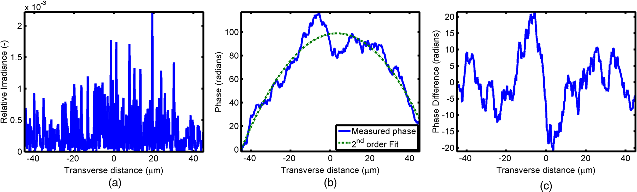 A second-order polynomial is fitted to the data utilizing least squares,19 which represents a spherical wavefront having a source near the origin and has a radius of curvature of 98.6 μm. As one would expect, the wavefront differs from this quadratic curvature due to scattering. The difference between the measured phase and polynomial is shown in Fig. 4(b). The sidebands, discussed in Sec. 3, are then isolated by demodulating the measured signals, as discussed in Sec. 3.2. The relative demodulated probe power is shown in Fig. 5(a), and its phase is shown in Fig. 5(b) in blue. The radius of curvature is found to be 66.9 μm. The smaller radius of curvature indicates that the wavefront is centered in the medium closer to the US waist. The difference between the measured phase and the second-order polynomial varies by radians and is illustrated in Fig. 5(c). Fig. 5(a), Irradiance of the demodulated optical signal normalized by the source power. (b), The phase of the demodulated optical signal. The phase (blue) is fitted with a second-order polynomial (green) with a radius of curvature of 66.9 μm. (c), The difference between the demodulated phase and the second-order fit. 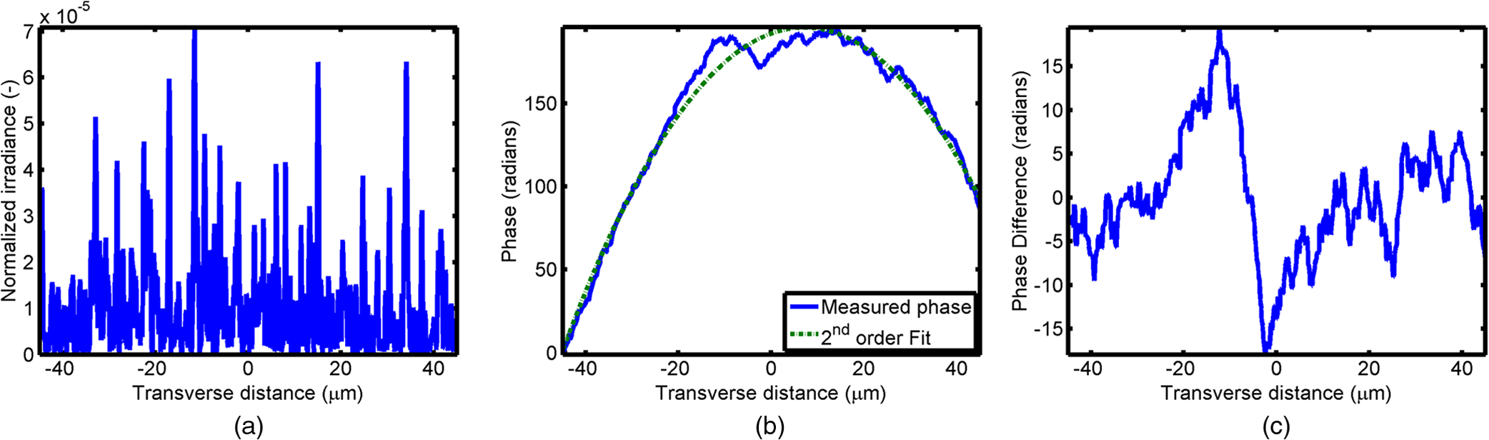 Delivery waves are created from the phase conjugate carrier and sidebands and simulated in the synthetic tissue. The results [Fig. 6(a)] show that the PCS delivery wave exhibits strong focusing at the US guidestar position. The energy is highly localized in the horizontal, and less so in the vertical axis. These results agree with experimental results.4 The PCC [Fig. 6(b)] retraces its path through the medium and converges back to the probe beam source. This is because the signal is the phase conjugate of the probe beam. Phase conjugation forces it to retrace its path through the scattering medium. Fig. 6Phase conjugate carrier and sidebands in the synthetic tissue model. The model indices of refraction are illustrated in gray, the US beam is in green, and the optical field is in red.  To evaluate the performance of the guidestar, a measure of energy concentration is needed. We propose a metric that is independent of the source power. The time-averaged energy within the medium is normalized by the optical input power. The time-averaged energy is computed as where the integral is calculated over a volume, , defined by a cylinder of radius, . The cylinder is centered at the US beam focal point and, like the simulated medium, extends 1 m in the third dimension. An example of this cylinder may be found in Fig. 7(b). We note that the integrand in Eq. (4) is the fluence rate from diffusive optical tomography, so the integral is proportional to the power that would be absorbed by a weakly absorbing medium in the indicated volume. The permittivity of the medium, , is related to the index of refraction by where is the free space permittivity. The volume integral is normalized by the source power, resulting in an energy-to-input-power (EP) ratio with units of femtoseconds. The EP ratio is calculated for cylinders of increasing radii, and the results are plotted to provide a measure of how the EP ratio varies over radial distance from the ultrasound beam waist. The result for the phase conjugate sideband and carrier signals are shown on a log-log scale in Fig. 7(b). The graph illustrates that the EP ratio is higher for the PCS signal near the center of the US beam, indicating a greater amount of energy focusing than is achieved by the PCC. As the distance from the center of the US beam grows, the amount of energy in either beam becomes similar and indicates that the energy in the PCS beam is concentrated at the US focus. To compute the actual amount of energy within the medium, one simply needs to multiply the EP ratio by the desired input power.Fig. 7The energy-to-input-power ratio for the focused (green solid) and unfocused (blue dashed) delivery waves on a log-log scale. The values are plotted for growing distances from the center of the US beam (shown as R).  To further investigate the focusing of the PCS beam, the time-averaged Poynting vector is calculated and illustrated in Fig. 8 for the probe beam [Fig. 8(a)], PCS [Fig. 8(b)], and PCC [Fig. 8(c)]. The direction of the Poynting vector is illustrated with color, where red indicates the vector is directed down along the depth axis and cyan indicates a vector in the opposite direction. The magnitude of the Poynting vector (irradiance) is utilized as an intensity envelope for the figure. Pixels with a higher intensity correspond to higher irradiance values. The pixels containing a magnitude below a threshold are set to white. The optical channeling phenomenon is visible. These graphs illustrate that the power is traveling along these channels with little divergence. Fig. 8The angle of the Poynting vector is utilized to create an image where cyan suggests the vector is directed down along the depth axis and red suggests the opposite direction. The magnitude is utilized as an intensity envelope for the figure. Pixels with a higher intensity correspond to higher magnitude values.  4.2.Scattering PhantomThe same process is repeated for the titanium oxide phantom containing random scatterers. A 532-nm probe beam interrogates the medium as shown in Fig. 2. As before, the field is measured at the detector (position is indicated by the yellow line) for four US phases. The received signal is demodulated to isolate the sidebands, and Fig. 9 shows the resulting amplitude [Fig. 9(a)] and phase [Fig. 9(b)]. A second-order polynomial is also fitted to the unwrapped phase (green). The difference between actual phase and the fitted second-order function is shown in Fig. 9(c) and is larger than the previous example owing to the high scattering. Fig. 9(a), Irradiance of the US-demodulated optical signal normalized by the source power for an example titanium oxide phantom. (b), The phase of the demodulated signal. Note the phase (blue) is fitted with a second-order polynomial (green) with a radius of curvature of 57.5 μm. (c), Difference between the demodulated phase and the second-order fit.  It is well known that energy can be directed to some extent by focusing into tissue, as is done in confocal microscopy. To prove that the phase conjugation results here could not be achieved just by focusing, a delivery signal is created with a phase given by the second-order curve shown in Fig. 9(b), and the amplitude is unchanged. If we removed the scatterers, this beam, the phase conjugate fit (PCF), should focus to a point. The PCF wavefront is simulated as a delivery wave along with the phase conjugate sideband and carrier waves (Fig. 10). Recall, the phase conjugate carrier is the phase conjugate of the unmodulated probe beam. That signal [Fig. 10(a)] travels back to the source, as expected. The phase conjugate fit [Fig. 10(c)] exhibits some focusing in the medium, but the spot is very broad due to the scattering. However, the phase conjugate sideband [Fig. 10(b)] focuses to a tight spot within the US beam width despite the high scattering. This comparison demonstrates that the high irradiance of light delivery is the result of phase conjugation, and not merely focusing. It is also interesting to note that the optical channeling effect is still present even after the signal has traveled a mean free path in the medium. Fig. 10The phase conjugate carrier (a), phase conjugate sideband (b), and phase conjugate fit (c) delivery waves in an example titanium oxide phantom. The US beam is illustrated in green, the medium of random scatterers in gray, and the electric field in red.  The Poynting vectors are computed in in a similar manner as above for the phase conjugate carrier and sideband, and fitted fields are shown in Fig. 11. The results show that the PCF and PCC signals exhibit little focusing. The PCS exhibits a converging energy density at the beam waist that quickly diverges beyond it. Figure 10 illustrates the resulting EP metric for each signal on a log-log plot. The EP ratio is lowest for the PCC (green dotted line), but it is interesting to note that the phase conjugate fit (blue dashed line) has about the same ratio as the PCS signal near the center of the US beam. This appears to contradict the field and Poynting vector distributions in the medium. However, the ultrasound beam radius is 3.72 μm (indicated by the vertical cyan line in Fig. 12); the energy delivered to the US beam is 2.6 times higher for the PCS than the phase conjugate fit signal. This suggests that the heterogeneity of the optical channels is skewing the result for small distances. As discussed earlier, phase conjugation can achieve suboptical wavelength resolution through the diffusive lens effect.3 However, the US guidestar cannot select the location for this focusing to an accuracy less than the US resolution. Therefore, we shall use the radius of 3.72 μm to characterize the enhancement. Note that the EP ratio (energy for a given input power) for optical phase conjugation with a US guidestar drops as the opacity of the medium increases. This agrees with previously reported experimental results16 as well as other results obtained from other computational models.5 It is important to remember that these simulations allow for variation in two dimensions. Although we do not have 3-D simulation data, geometric arguments suggest that the enhancement would be squared in three dimensions. In our example, the enhancement by a factor of 2.7 in 2-D means the focused energy will be times greater than the phase conjugate fit signal in three dimensions. 5.ConclusionsWe have shown through computational modeling that the depth to which light can be focused in a turbid medium can be enhanced through phase conjugation using an ultrasound-generated guidestar. We performed computations using a 2-D FDTD simulation of the optical wave propagating in a medium with a heterogeneous index of refraction. Two cases have been simulated. The first utilizes optical properties typical of biological tissue and homogeneous acoustic properties. The US is a focused Gaussian wave that produces pressure-induced changes in the index of refraction. The second is a highly scattering medium similar to a gel containing titanium oxide particles with a small cylindrical region modulated at the US frequency. In both cases, the guidestar wavefront is computed from the US sidebands of the detected light. Light is delivered to the focus of the US wave more effectively using the phase-conjugate of the guidestar wave than it is by attempting to focus the optical wavefront to the same point. The FDTD simulations suggest the presence of spatially coherent optical channels within a turbid medium. These optical channels have been noted elsewhere17 for a 2-D simulation, and they appear to exist in one 3-D simulation.18 However, there is a dearth of information about the optical channeling effect in three dimensions. Furthermore, different 2-D simulations show different results, and the behavior of the channels depends on the exact scattering structures, their densities, and the depth of the medium. Understanding these optical channels in two and three dimensions is important because they retain their spatial coherence well beyond the distance predicted by diffraction and may present a method for localizing power within the medium. AcknowledgmentsC. DiMarzio and J. Hollmann acknowledge support from CenSSIS, the Gordon Center for Subsurface Sensing and Imaging Systems, under the Engineering Research Centers Program of the National Science Foundation (award number EEC-9986821). R. Horstmeyer acknowledges support from the National Defense Science and Engineering Graduate fellowship awarded through the Air Force Office of Scientific Research. ReferencesX. XuH. LiuL.V. Wang,
“Time-reversed ultrasonically encoded optical focusing into scattering media,”
Nat. Photon., 5
(1), 154
–157
(2011). http://dx.doi.org/10.1038/nphoton.2010.306 1749-4885 Google Scholar
J. L. HollmannC. A. DiMarzio,
“Modeling optical phase conjugation of ultrasonically encoded signal utilizing finite-difference time-domain simulations,”
Proc. SPIE, 8227 82270I
(2012). http://dx.doi.org/10.1117/12.907084 PSISDG 0277-786X Google Scholar
I. M. VellekoopA. LagendijkA. P. Mosk,
“Exploiting disorder for perfect focusing,”
Nat. Photon., 4
(5), 320
–322
(2010). http://dx.doi.org/10.1038/nphoton.2010.3 1749-4885 Google Scholar
Y. M. Wanget al.,
“Deep-tissue focal fluorescence imaging with digitally time-reversed ultrasound-encoded light,”
Nat. Commun., 3 928
(2012). http://dx.doi.org/10.1038/ncomms1925 NCAOBW 2041-1723 Google Scholar
S. H. TsengC. Yang,
“2-D PSTD simulation of optical phase conjugation for turbidity suppression,”
Opt. Express, 15
(24), 16005
–16016
(2007). http://dx.doi.org/10.1364/OE.15.016005 OPEXFF 1094-4087 Google Scholar
K. Yee,
“Numerical solution of initial boundary value problems involving Maxwell’s equation in isotropic media,”
IEEE Trans. Antenn. Propagat., 40
(3), 1068
–1075
(1966). http://dx.doi.org/10.1109/8.166532 IETPAK 0018-926X Google Scholar
B. SimonC. A. DiMarzio,
“Simulation of a theta line-scanning confocal microscope,”
J. Biomed. Opt., 12
(6), 064020
(2007). http://dx.doi.org/10.1117/1.2821425 JBOPFO 1083-3668 Google Scholar
M. N. O. Sadiku, Numerical Techniques in Electromagnetics, 2nd ed.CRC Press, Boca Raton, FL
(2000). Google Scholar
G. Mur,
“Absorbing boundary conditions for the finite-difference approximation of the time-domain electromagnetic-field equations,”
IEEE Trans. Electromag. Compat., EMC-23
(4), 377
–382
(1981). http://dx.doi.org/10.1109/TEMC.1981.303970 IEMCAE 0018-9375 Google Scholar
L. V. Wang,
“Mechanisms of ultrasonic modulation of multiply scattered coherent light: an analytic model,”
Phys. Rev. Lett., 87
(4), 043903
(2001). http://dx.doi.org/10.1103/PhysRevLett.87.043903 PRLTAO 0031-9007 Google Scholar
C. V. RamanN. S. N. Nath,
“The diffraction of light by high frequency sound waves: part I,”
Proc. Ind. Acad. Sci., 3
(5), 406
–412
(1936). PISAA7 0370-0089 Google Scholar
B. SimonC. A. DiMarzio,
“Simulation of imaging with a theta line-scanning confocal microscope,”
Proc. SPIE, 6861 68610V
(2008). http://dx.doi.org/10.1117/12.764146 PSISDG 0277-786X Google Scholar
A. DunnR. Richards-Kortum,
“Three-dimensional computation of light scattering from cells,”
IEEE J. Sel. Top. Quant. Electr., 2
(4), 898
–905
(1996). http://dx.doi.org/10.1109/2944.577313 IJSQEN 1077-260X Google Scholar
H. KogelnikT. Li,
“Lasers and resonators,”
Appl. Opt., 5
(10), 1550
–1567
(1966). http://dx.doi.org/10.1364/AO.5.001550 APOPAI 0003-6935 Google Scholar
I. M. VellekoopA. P. Mosk,
“Focusing coherent light through opaque strongly scattering media,”
Opt. Lett., 32
(16), 2309
–2311
(2007). http://dx.doi.org/10.1364/OL.32.002309 OPLEDP 0146-9592 Google Scholar
E. J. McDowellet al.,
“Turbidity suppression from the ballistic to the diffusive regime in biological tissues using optical phase conjugation,”
J. Biomed. Opt., 15
(16), 025004
(2010). http://dx.doi.org/10.1117/1.3381188 JBOPFO 1083-3668 Google Scholar
W. Choiet al.,
“Transmission eigenchannels in a disordered medium,”
Phys. Rev. B, 83
(13), 134207
(2011). http://dx.doi.org/10.1103/PhysRevB.83.134207 PRBMDO 0163-1829 Google Scholar
M. S. StarostaA. K. Dunn,
“Three-dimensional computation of focused beam propagation through multiple biological cells,”
Opt. Express, 17
(15), 12455
–12469
(2009). http://dx.doi.org/10.1364/OE.17.012455 OPEXFF 1094-4087 Google Scholar
D. C. MontgomeryE. A. PeckG. G. Vining, Introduction to linear regression analysis, Wiley, New York City, New York
(2001). Google Scholar
|