1.

Introduction

Diffuse optical tomography (DOT)^1–6 is one of the emerging noninvasive functional imaging modalities.^1,3 To study the regional physiological process in highly scattering media such as tissue, a low-energy, near infrared (NIR) light-based imaging technique is one of the best in terms of quantitative recovery of spectroscopic optical parameters. The main goal is to recover the spatial variation of optical properties, which can be used to diagnose the different metabolic states of tissue. An iterative reconstruction algorithm^1–3 attempts to recover the optical properties such as absorption (${\mu }_a$) and reduced scattering coefficients (${\mu }_s^{\prime }$) by repeatedly solving the forward problem and updating ${\mu }_a$ and ${\mu }_s^{\prime }$ based on the difference between measurement data and the forward prediction. System calibration is an important issue in a variety of applications such as DOT imaging,^7–14 fluorescence imaging,¹⁵ electrical impedance tomography,¹⁶ photoacoustic tomography,¹⁷ ultrasound assisted optical imaging, thermal imaging, and defect detection in civil engineering. The reconstruction depends on experimental measurements, and the iteration is continued until the experimental measurement matches the forward prediction. In DOT, the data calibration is often performed using a homogeneous reference phantom.^8–14 Tarvainen et al.⁹ have discussed a calibration strategy with homogeneous data. One way to compensate for the measurement error is to use difference imaging, which is known to produce images with few artifacts.^8,9 However, this method cannot be used when absolute optical properties are required or when a reference measurement is not available. We need to devise ways to obviate the need for a “background” homogeneous data set for the difference imaging approach. That said, the focus of this study is to estimate a background image for difference imaging without taking a separate background measurement. The calibrated absolute flux density by adequately modeling the measurement process by either analytic or numerical methods is a must for good reconstructed images.^8–14 In DOT imaging, total flux ($U_{\text{measured}}$) measured by a detector over a finite area has to be calibrated to account for the system response function ($R$) before it is plugged into the optimization algorithm. The estimation of response functions that comprises the quantum conversion efficiency ($Q$) of the photo multiplier tube (PMT), coupling factor ($C$), laser source strength ($S$), fiber loss ($L$), free propagation of light ($\mathrm{\Gamma }$),⁴ and transfer function ($H$) of the measurement system is quite tedious. Calibrating the measurement data to account for all these aberrations is an iterative method^4,13 where estimating flux density ($J_n$) (see Ref. 4) requires the inversion of Eq. (2) with the prior information of all instrumental response functions.^8,13 The calibration process requires experimental homogeneous data (measurement data with a homogeneous phantom),^8,9,12,13 instrument calibration, and various offset terms.^8,9,11,13

In this context, we modified Eq. (3) of Ref. 4 by incorporating various instrumental response functions ($R$) and arrived at a simple absolute flux density estimation scheme [Eqs. (1)–(6)] (Scheme 1) that uses homogeneous measurement data ($U_{\text{measured}}^{\mathrm{homo}}$) and a background optical parameter, which is measured by a standard method.¹⁸ We reconstructed the absolute optical property of pork tissue phantom, human tissue, and tissue-mimicking phantoms.

However, in practical situations such as in a clinical application, the homogeneous measurement data will not be available. For such situations, a scheme (Scheme 2) is proposed to estimate a homogeneous data from a heterogeneous phantom measurement. In such a scheme, the homogeneous data are estimated ($U_{\text{measured}}^{\mathrm{est}-\mathrm{homo}}$) by statistically averaging the heterogeneous measurement data ($U_{\text{measured}}^{\mathrm{hetero}}$) and redistributing them to the corresponding detector positions [Eq. (7)]. The estimated homogeneous ($U_{\text{measured}}^{\mathrm{est}-\mathrm{homo}}$) data is used^13,19 to estimate the initial background optical parameters and the flux density [Eq. (8)]. Using this approach, we reconstructed absolute optical property distribution of tissue-mimicking phantoms, pork tissue, and human tissue.

2.

Calibration of Measurement Data

2.1.

Calibration of Heterogeneous Measurement Data Using Homogeneous Data

The transport of light through a diffusive medium such as tissue is modeled through the diffusion equation,^2,3 given as $[-\nabla ·\kappa (r)\nabla +{\mu }_a(r)]\mathrm{\Phi }(r)=S(r)$, where $\kappa (r)=1/3[{\mu }_a(r)+{\mu }_s^{\prime }(r)]$. The forward model is solved² over the domain (V) to estimate the flux density (${\mathrm{\Phi }}^{\text{predicted}}=\mathcal{M}[\mathrm{\Phi }]$) on the surface boundary ($\mathrm{\Omega }$). $\mathcal{M}:L_2(V)\to L_2(\mathrm{\Omega })$ is the measurement operator. Due to the spatial ($r\in V$, $\mathrm{\Omega }$) variation of the optical parameter $[\mathrm{\Delta }{\mu }^i(r)]$, the perturbation equation in terms of the optical parameter can be written in a Taylor series expansion, retaining only the first derivative, as²⁰

Eq. (1)

$$\begin{gathered} \mathrm{\Delta }{M}^i={\mathrm{\Phi }}_{\text{measured}}^{\mathrm{cal}}-{\mathrm{\Phi }}^{\text{predicted}(i)}=F^{\prime }({\mu }^i)[\mathrm{\Delta }{\mu }^i] \\ {\mu }^{i+1}(r)={\mu }^i(r)+\mathrm{\Delta }{\mu }^i(r), \end{gathered}$$

where ($F^{\prime }$) is the Jacobian matrix [1, 3, 20] of forward operator $F$, $\mathrm{\Delta }{M}^i$ is the difference between the calibrated experimental flux density (${\mathrm{\Phi }}_{\text{measured}}^{\mathrm{cal}}$) and the forward model predicted flux density (${\mathrm{\Phi }}^{\text{predicted}(i)}$) at the $i$’th iteration. Now, we will present a few mathematical equations by which flux density will be estimated from total detected flux, $U_{\text{measured}}$.

The free space light propagation [Fig. 1(a)] from phantom surface to detector⁴ is given as

$$\mathrm{\Gamma }(r,r_d)=\xi (r,r_d)\frac{f(\mathrm{NA}-\sin {\theta }_d)}{{|r_d-r|}^2}\cos \theta \cos {\theta }_{d}dA,$$

where $r=|\overrightarrow{r^{\prime }}-\overrightarrow{r^k}|$, [$r_k$, $r^{\prime }\in V$, $\mathrm{\Omega }$], $\xi (r,r_d)$ is the visibility factor, $\cos \theta =\widehat{\zeta }.\widehat{n}$ is the cosine dependent on Lambert’s law, $\widehat{\zeta }$ is the power radiation direction on surface $\mathrm{\Omega }$, NA is the numerical aperture of fiber, ${\theta }_d$ is the detector orientation with respect to the line of sight, and $r_d$ is the distance between detector and surface ($\mathrm{\Omega }$) (see Ref. 4). With an inhomogeneity of $\mathrm{dia}=2r^{\mathrm{incl}}$ with $({\mu }_a^{\mathrm{incl}},{\mu }_s^{\prime \mathrm{incl}})$ embedded in the homogeneous phantom, the total flux over the fiber cross-section ($dA$) measured by the lock-in amplifier can be written as

Eq. (2)

$${}^{k,d}{U}_{\text{measured}}^{\mathrm{hetero}}=\frac{Q^{k,d}·H^{k,d}·L^{k,d}}{\pi }{\int }_{\mathrm{\Omega }}{C}^{k,d}(r,r_d)J_n^{k,d}(S_k,r){\mathrm{\Gamma }}^{k,d}(r,r_d)\mathrm{d}\mathrm{\Omega },$$

where $({\mu }_a,{\mu }_s^{\prime })=({\mu }_a^0,{\mu }_s^{\prime 0})\cup ({\mu }_a^{\mathrm{incl}},{\mu }_s^{\prime \mathrm{incl}})$ and $J_n^{k,d}(S_k,r)$, is the outgoing normal flux density at the surface ($d\mathrm{\Omega }$) of the phantom for a particular source position $k$ ($S_k$, $k=1\dots N=12$) and detector position $d$ ($D_d$, $d=-m\dots m$). For a medium with a homogeneous distribution of ${\mu }_a^0$, ${\mu }_s^{\prime 0}$ over the domain, the outgoing normal flux density at the surface is $J_{n,0}^{k,d}(S_k,r)$ and the total flux measured by the lock-in amplifier can be written as

Eq. (3)

$${}^{k,d}{U}_{\text{measured}}^{\mathrm{homo}}=\frac{Q^{k,d}·H^{k,d}·L^{k,d}}{\pi }{\int }_{\mathrm{\Omega }}{C}^{k,d}(r,r_d)J_{n,0}^{k,d}(S_k,r){\mathrm{\Gamma }}^{k,d}(r,r_d)\mathrm{d}\mathrm{\Omega }.$$

Fig. 1

(a) Experimental model; (b) simulated domain and data collection model; (c) source strength versus flux density at detector $D_{d=3}$. The source intensity is given over a single boundary element, and detection has taken place at the boundary node.

Scaling the experimentally measured heterogeneous data (${}^{k,d}{U}_{\text{measured}}^{\mathrm{hetero}}$) by ${\mathrm{\Phi }}^{\text{predicted}(0)}/{}^{k,d}{U}_{\text{measured}}^{\mathrm{hom}\mathrm{o}}$ where (${}^{k,d}{U}_{\text{measured}}^{\mathrm{hom}\mathrm{o}}$) is the experimentally measured homogeneous data for source $k$ and detector $d$ position, the calibrated experimental heterogeneous flux (${\mathrm{\Phi }}_{\text{measured}}^{\mathrm{cal}\mathrm{hetero}}$) can be written for the $k$’th source and the $d$’th detector as

Eq. (4)

$$\begin{gathered} {}^{k,d}{\mathrm{\Phi }}_{\text{measured}}^{\mathrm{cal}\mathrm{hetero}}=\frac{{}^{{}^{k,d}{U}_{\text{measured}}^{\mathrm{hetero}}}}{{}^{k,d}{U}_{\text{measured}}^{\mathrm{homo}}}\times {}^{k,d}{\mathrm{\Phi }}^{\text{predicted}(0)}(r) \\ =\frac{\frac{Q^{k,d}·H^{k,d}·L^{k,d}}{\pi }{\int }_{\mathrm{\Omega }}{C}^{k,d}{S}_k{J}_n^{k,d}(r){\mathrm{\Gamma }}^{k,d}\mathrm{d}\mathrm{\Omega }}{\frac{Q^{k,d}·H^{k,d}·L^{k,d}}{\pi }{\int }_{\mathrm{\Omega }}{C}^{k,d}{S}_k{J}_{n,0}^{k,d}(r){\mathrm{\Gamma }}^{k,d}\mathrm{d}\mathrm{\Omega }}\times {\mathrm{\Phi }}^{\text{predicted}(0)}(r), \end{gathered}$$

where we used the property $J_n\propto S_k$ (when other parameters are fixed) [Fig. 1(b) and 1(c)]. With known background optical parameters $({\mu }_a^0,{\mu }_s^{\prime 0})$, the simulated homogeneous flux density (at iteration $i=0$) at the surface can be written as ${\mathrm{\Phi }}^{\text{predicted}(0)}(r)=J_{n,0}^{k,d}$. We make an assumption that when ($dA\ll \mathrm{\Omega }$), the system transfer function does not vary over the cross-section of the fiber bundle (either with or without inhomogeneity) and the calibrated flux density then can be written as

Eq. (5)

$${}^{k,d}{\mathrm{\Phi }}_{\text{measured}}^{\mathrm{cal}}=\frac{\frac{Q^{k,d}·H^{k,d}·L^{k,d}}{\pi }}{\frac{Q^{k,d}·H^{k,d}·L^{k,d}}{\pi }}\times \frac{C^{k,d}{S}_k{\mathrm{\Gamma }}^{k,d}\mathrm{\Omega }{J}_n^{k,d}(r)}{C^{k,d}{S}_k{\mathrm{\Gamma }}^{k,d}\mathrm{\Omega }{J}_0^{k,d}(r)}\times J_{n,0}^{k,d}(r)\mathrm{.}$$

The calibrated experimental heterogeneous flux density for the $k$’th source and the $d$’th detector is reduced to

Eq. (6)

$${}^{k,d}{\mathrm{\Phi }}_{\text{measured}}^{\mathrm{cal}\mathrm{hetero}}=J_n^{k,d}.$$

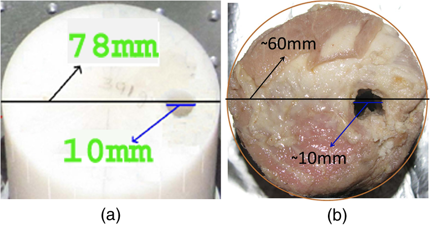
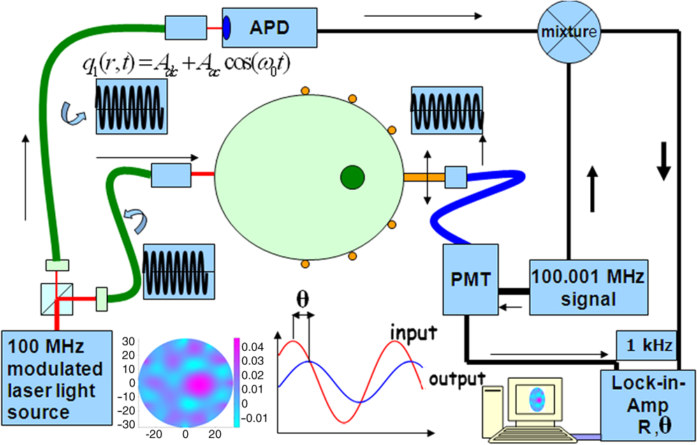
3.

Simulation Results

A simulated phantom with a diameter of 80 mm ($2R\prime$) with background ${\mu }_a^0=.005{\mathrm{mm}}^{-1}$, ${\mu }_s^{\prime 0}=0.83{\mathrm{mm}}^{-1}$ [similar to the phantom in Fig. 2(a)] is used for generating²⁰ the simulated homogeneous flux density ${\mathrm{\Phi }}_{\mathrm{sim}}^{\mathrm{homo}}$. We discretized the simulated phantom domain into 4032 elements and 2089 nodes and the finite element method (FEM) solution of light diffusion is obtained all over the domain.² Seven detector measurements at boundary nodes are taken (flux density) for each of the source locations [as shown in Fig. 1(b)]. An inhomogeneity (an object) with a diameter of 8.2 mm (full width at half maximum) having ${\mu }_a^{\mathrm{incl}}=.015{\mathrm{mm}}^{-1}$ and the same value of ${\mu }_s^{\prime }$ as background is introduced at (19.2,0) to generate a simulated heterogeneous flux density (${\mathrm{\Phi }}_{\mathrm{sim}}^{\mathrm{hetero}}$) [Fig. 3(a)].

Fig. 2

(a) The tissue-mimicking phantom; (b) the pork tissue phantom.

Fig. 3

(a) Simulated heterogeneous (blue line) and homogeneous (red line) flux densities, (b) simulated heterogeneous (blue line) and estimated homogeneous (red line) flux densities from the heterogeneous flux density [Eq. (8)], (c) the perturbation in data due to inclusion when the perturbation is measured with respect to the true homogeneous flux density, (d) the perturbation in data due to inclusion when the perturbation is measured with respect to the estimated homogeneous flux density.

The homogeneous flux density is estimated (${\mathrm{\Phi }}_{\mathrm{sim}}^{\mathrm{est}-\mathrm{homo}}$) [Fig. 3(b)] from simulated heterogeneous flux density (${\mathrm{\Phi }}_{\mathrm{sim}}^{\mathrm{hetero}}$) by the proposed method [Eq. (7)]. The perturbation or mismatch ($\mathrm{\Delta }M$) of the flux density with inclusion is shown in Fig. 3(c) and 3(d), when the perturbation/mismatch of fluence is measured with respect to true homogeneous flux density ($\mathrm{\Delta }{M}_t={\mathrm{\Phi }}_{\mathrm{sim}}^{\mathrm{hetero}}-{\mathrm{\Phi }}_{\mathrm{sim}}^{\mathrm{homo}}$) and with estimated homogeneous flux density $\mathrm{\Delta }{M}_{\mathrm{est}}={\mathrm{\Phi }}_{\mathrm{sim}}^{\mathrm{hetero}}-{\mathrm{\Phi }}_{\mathrm{sim}}^{\mathrm{est}-\mathrm{homo}}$, respectively. The deviation of absolute mismatch ($\mathrm{\Delta }M$) is shown in Fig. 4, when we use the estimated homogeneous data. The mean error between the simulated homogeneous data and estimated homogeneous data $\overline{e}={\sum }_{i=1}^{84}|({\mathrm{\Phi }}_{\mathrm{sim}}^{\mathrm{hetero}}-{\mathrm{\Phi }}_{\mathrm{sim}}^{\mathrm{est}-\mathrm{homo}})/{\mathrm{\Phi }}_{\mathrm{sim}}^{\mathrm{homo}}|/84$ is found to be $\overline{e}\simeq 0.004$, which validates the homogeneous data estimation algorithm [Eq. (7)]. We have also placed multiple inhomogeneities (2) at (19.2,0) and (0,19.2), (3) at (19.2,0), ($-19.2$, 0) and (0, 19.2) and estimated ${\mathrm{\Phi }}_{\mathrm{sim}}^{\mathrm{est}-\mathrm{homo}}$ from ${\mathrm{\Phi }}_{\mathrm{sim}}^{\mathrm{hetero}}$. The error is found to be low. The observations are tabulated for both trial and error, and effective perturbation (EP) strategies in Tables 1 and 2, respectively. The recovered absorption coefficients are obtained as 62%, 58%, and 61% of the original contrast, respectively. We have observed noisy images as the number of inclusions increases.

Fig. 4

The deviation of absolute mismatch ($\mathrm{\Delta }M$) when the perturbation/mismatch is obtained using estimated homogeneous flux density.

4.

Experimental System and Phantom Preparation

A frequency domain noncontact DOT imaging system is designed and fabricated (Figs. 5 and 6) for conducting the experiment. A single-laser light source is used to irradiate the phantom, and a single detector moves around the phantom for collecting the exiting photon from the tissue boundary.^20,21,22 The light source is an intensity-modulated laser diode (HL7851G, Thorlabs, Newton, New Jersey), at a wavelength of 830 nm, of average power 4.3 mW, whose modulation frequency is 100 MHz. The diode is driven by a 50-mA DC current mixed with a 20 mA radio-frequency (rf) current on a Thorlabs TCLDM9 laser mount. The rf signal is from an ultrastable function generator (Tektronix AFG 3102, Tektronix, Beaverton, Oregon). In order to have a stable wavelength output, the laser diode is cooled by a Thorlabs TCM1000T cooler. The output from the laser diode is split using a 10:1 beam-splitter. The less-intense beam is fed to an avalanche photo-diode (APD) to generate a 100-MHz reference signal, and it is used as an input to the mixer (Fig. 5). The second input to the mixer is a 100.001-MHz rf signal from same function generator. The 1-KHz beat signal from the mixer output is used as a reference signal for the lock-in amplifier. The intense part of the light from the beam-splitter is coupled to a 3-mm diameter multimode fiber to illuminate the phantom and the exiting light at the phantom boundary is collected by a fiber bundle with a 5-mm diameter, which subsequently transmits the light to a detector, an IR-sensitive PMT from Hamamatsu (Shizuoka, Japan), which is gain-modulated at 100.001 MHz for our application. The dynode of the PMT is driven by a 100.001-MHz sinusoidal signal (second channel of Tektronix AFG 3102). The heterdyne signal of 1 KHz from the detector is fed to a lock-in amplifier, which also receives the reference signal from the APD. This facilitates the measurement of the exiting photon signal from the PMT. We have collected a set of 84 amplitude measurements (12 equally spaced source positions spanning the phantom surface multiplied by 7 detector measurements per source location).

Fig. 5

Schematic model for a frequency domain DOT imaging system.

Fig. 6

The frequency domain experimental setup for DOT data measurements.

The phantom is an artificial tissue-mimicking object whose background optical properties are similar to those of a tissue. They are fabricated²³ to mimic the absorption and scattering properties of the tissue. The cylindrical phantom is made of Araldite and a hardener whose scattering and absorption properties are tailored by mixing titanium dioxide powder and India ink, respectively. Here, 400 g of resign (C-51 Araldite resign, Atul Polymer, India) and India ink (0.25 ml 2%) are mixed thoroughly together with 1.3 g titanium dioxide until all the gas is released. Initially, 20 g of hardener (50% of total volume) is added to the mixture and mixed well, especially at the bottom. After proper mixing, the rest of the hardener is added to the main content and mixed thoroughly for 1 h until it gets hot and starts cooling down. Once the phantom is hardened enough, it is machined to cylindrical shape.

5.

Experimental Results and Discussion

An NIR laser light modulated by a 100-MHz sinusoidal signal is used to estimate the background optical parameter by measuring the diffuse reflected photon at several locations away from the source.^18,20 The measured background absorption and scattering coefficient of an experimental tissue-mimicking phantom are found to be ${\mu }_a=0.005{\mathrm{mm}}^{-1}$ and ${\mu }_s^{\prime }=0.83{\mathrm{mm}}^{-1}$ for the phantom shown in Fig. 2(a). Absorption and scattering coefficients of the phantom shown in Fig. 7(a) is found to be ${\mu }_a=0.002{\mathrm{mm}}^{-1}$ and ${\mu }_s^{\prime }=1.21{\mathrm{mm}}^{-1}$, respectively. A small cylinder is drilled in the homogeneous phantom and is filled with 10% intralipid solution and India ink²⁴ to provide the inhomogeneous regions.

Fig. 7

(a) Two embedded inhomogeneities of 12 mm and 10 mm in diameter in a phantom of 60.6 mm diameter, 70.5 mm height. (b) Reconstructed image from calibrated data using measured heterogeneous data (using method 2). (c) The contrast variation along the cross-sectional line through the inhomogeneities (blue line) in the phantom. The line plot (purple dotted line) through the center of inhomogeneities of the reconstructed image shown in (b).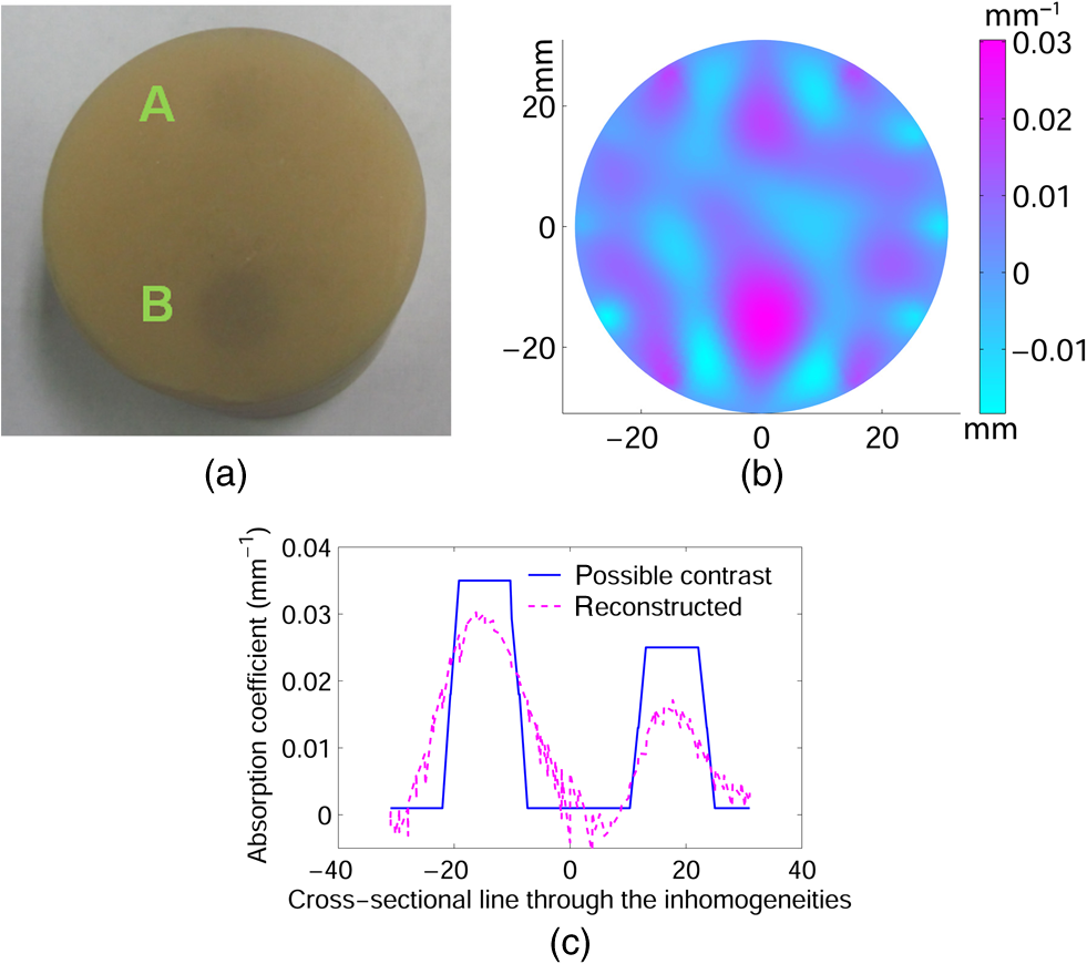

The frequency domain experimental setup is shown in Fig. 6. Experiments have been carried out for both regularly and irregularly shaped phantoms [Fig. 2(a) and 2(b)]. A cylindrical tissue-mimicking phantom (78 mm diameter, ${\mu }_a=0.005{\mathrm{mm}}^{-1}$, ${\mu }_s^{\prime }=0.83{\mathrm{mm}}^{-1}$) [Fig. 2(b)] and an irregular cylindrical ($\mathrm{dia}\approx 60\mathrm{mm}$) pork flesh [Fig. 2(b)] (as a biological phantom) have been used. For the pork tissue phantom, because of the irregularity, the distance ($r_d$) from the detector to the sample surface varies from $1\mathrm{mm}\le$ to $\le 5\mathrm{mm}$. A 10-mm diameter inhomogeneity (${\mu }_a^{\mathrm{incl}}\simeq 0.03{\mathrm{mm}}^{-1}$, made of ink, water, and intralipid)²⁴ is introduced to a tissue-mimicking phantom [Fig. 2(a)] and approximately 10 mm of fat is introduced inside the pork tissue (see Ref. 25 and Table 2) (${\mu }_a=0.006{\mathrm{mm}}^{-1}$, ${\mu }_s^{\prime }=0.67{\mathrm{mm}}^{-1}$).

We experimentally measured the exiting light amplitude for homogeneous ($U_{\text{measured}}^{\mathrm{homo}}$) and heterogeneous ($U_{\text{measured}}^{\mathrm{hetero}}$) phantoms by moving the detector over a constant radius. The theoretical flux density for homogeneous phantom and the experimental calibrated flux density [Eq. (5)] using detected experimental homogeneous data for regular phantom are shown in Fig. 8. Using Eq. (7), we estimated experimental homogeneous data ($U_{\text{measured}}^{\mathrm{est}-\mathrm{homo}}$) from detected heterogeneous data ($U_{\text{measured}}^{\mathrm{hetero}}$), and our findings are shown in Fig. 9(a). The calibrated flux densities [for phantom Fig. 2(a)], obtained by Eqs. (4) and (7), are shown in Fig. 9(b). The perturbation of the flux density due to inclusion is shown in Fig. 9(c), when the perturbation ($\mathrm{\Delta }{M}_t$) is measured with respect to simulated homogeneous flux density and the calibration is carried out using an experimental homogeneous measurement. The perturbation of the flux density due to inclusion is shown in Fig. 9(d), when the perturbation ($\mathrm{\Delta }{M}_{\mathrm{est}}$) is measured with respect to simulated homogeneous flux density, and the calibration is carried out using estimated homogeneous measurement with Eq. (7). The deviation of absolute mismatch ($\mathrm{\Delta }M$) is shown in Fig. 10, when we use the estimated homogeneous measurement.

Fig. 8

Experimental calibrated heterogeneous flux density (blue line) when calibration is performed using experimentally detected homogeneous data [see Eqs. (3)–(6)]. The simulated homogeneous flux density is also shown (red line).

Fig. 9

(a) Experimentally detected heterogeneous data (${}^{k,d}{U}_{\text{measured}}^{\mathrm{homo}}$) (blue line) and estimated experimental homogeneous data (${}^{k,d}{U}_{\text{measured}}^{\mathrm{est}-\mathrm{homo}}$) (red line) using Eq. (7). (b) Experimental calibrated heterogeneous flux density (blue line) using Eqs. (7) and (8) and simulated homogeneous flux density (red line). (c) Calibration is carried out using experimental homogeneous measurement. (d) Calibration is carried out using an estimated experimental homogeneous measurement.

Fig. 10

The deviation of absolute mismatch when the perturbation/mismatch is obtained using an estimated homogeneous measurement.

The reconstructed image of a regular tissue-mimicking phantom when calibration is carried out with detected experimental homogeneous total flux and estimated total flux is shown in Fig. 11(a) and 11(b), respectively. The cross-section line plot through the inhomogeneity for both cases is shown in Fig. 11(c). The mean square error (MSE) with iteration is presented for both methods in Fig. 11(d). The results match very closely. The reconstructed image of the pork phantom, when calibration is carried out with experimental homogeneous total flux and estimated homogeneous flux, are shown in Fig. 12(a) and 12(b), respectively. The cross-section line plot through the inhomogeneity for both cases is shown in Fig. 12(c). Figure 12(d) shows the variation of the MSE with iteration. The reconstructed results with the estimated homogeneous data is bit noisy. This noise may be introduced during estimation due to more inhomogeneity in the background, as already analyzed and tabulated. For an irregular phantom, the small variation of geometrical shape matrix ($r_d$) may cause more inaccuracy in the homogeneous parameter estimation due to inappropriate free space photon propagation compensation.

Fig. 11

Reconstruction image of a tissue-mimicking phantom with an embedded inhomogeneity [Fig. 2(a)] when the calibration is performed (a) with experimentally detected homogeneous data (using method 1), (b) with estimated homogeneous data (using method 2) (c) The contrast through the cross-sectional line through the center of inhomogeneity. (d) The variation in MSE with iterations.

Fig. 12

(a) Reconstruction image of fat inserted inside the pork phantom when the calibration is performed with (a) experimentally detected homogeneous data (using method 1) and (b) estimated homogeneous data (method 2). (c) Cross-sectional line through the inhomogeneity. (d) The variation of MSE with iterations.

Experiments are carried out with two embedded inhomogeneities made of India ink and 10% intralipid. The reconstructed results using measured homogeneous and estimated homogeneous data are shown in Fig. 13(a) and Fig. 13(b), respectively.

Fig. 13

A phantom with two embedded inhomogeneities. The reconstructed results when the calibration is performed with (a) experimentally detected homogeneous data (using method 1) and (b) estimated homogeneous data (using method 2).

Apart from that, we used another 60-mm-diameter phantom [Fig. 7(a)] (background ${\mu }_a=0.002{\mathrm{mm}}^{-1}$, ${\mu }_s^{\prime }=1.21{\mathrm{mm}}^{-1}$), where there were two embedded inhomogeneities of different absorption coefficients. The experimental homogeneous data for this phantom is not available because the inhomogeneities were already inserted during phantom fabrication. We used the proposed method to estimate the homogeneous flux density for calibrating the heterogeneous measurements. The phantom image and reconstructed images are shown in Fig. 7(a) and 7(b). The cross-sectional line plot through the inhomogeneities is shown in Fig. 7(c). The results show that the homogeneous data estimation and image reconstruction is possible even without measured homogeneous data. This result validates the estimation algorithms.

The diffusion coefficient $\{\kappa (r)=1/3[{\mu }_a(r)+{\mu }_s^{\prime }(r)]\}$ distribution of the human hand has been reconstructed to demonstrate the ability of the proposed algorithm. The experimental homogeneous data from the hand phantom [Fig. 14(b)] is not available. Even when the measured homogeneous data is not available, we used the proposed “method 2” to estimate the homogeneous flux density for calibrating the heterogeneous measurements. The MR image and DOT reconstructed images are shown in Fig. 14(a) and 14(c), respectively. The locations of the bone in the hand are presented through the $\kappa (r)$ distribution. It shows that light cannot diffuse through the bone. The reconstructed image shows that there is more diffusion of light between the bones, where there are less dense tissue and more hollow spaces. The results with the pork tissue phantom and human hand image show that the homogeneous data estimation and absolute image reconstruction is possible in clinic, even when measured homogeneous data is available.

Fig. 14

(a) Cross-sectional MR image of a hand shows the bone locations. (b) Photograph of the hand-scanning DOT imaging system. (c) Reconstructed diffusion coefficient ($\kappa (r)$), when flux density is estimated using method (2). The diffusion through the bones is almost zero and shows the location of the bones.

6.

Conclusions

We have shown theoretically [Eqs. (3)–(8)] and experimentally that the proposed simple models estimate the absolute flux density ($\mathrm{\Phi }$) from detected total flux ($U_{\text{measured}}$). The estimated flux density with the proposed methods matches very closely with the simulated flux density. The reconstructed results for both the regular tissue-mimicking phantom and pork phantom are well resolved and localized when heterogeneous data is calibrated with experimentally measured homogeneous data. When the experimental homogeneous data are not available, the proposed statistical averaging method estimates the experimental homogeneous data from measured heterogeneous data and the MSE is found to be less than 0.005. The lower the effective perturbation is, the better the estimation is. The estimated homogeneous data match very closely to both theoretical and the experimental homogeneous data for a regular-shaped phantom [Fig. 2(a)]. Reconstructed results of a regular cylindrical phantom show similar results [Fig. 2(a)], when calibrated with and without prior knowledge of the experimental detected homogeneous data. However, the reconstructed result of the pork phantom matches closely when it is calibrated with estimated homogeneous data. Because of irregular shape of pork phantom, the distance between phantom surface and detector varies from 1 to 5 mm. The estimation of homogeneous data from heterogeneous data is carried out by projecting the photon flux from an irregular shape to a regular constant circular radius. $\mathrm{\Phi }$ varies nonlinearly with distance ($r$) and with optical parameters. The more irregular the phantom, the more discrepancy occurs in the calibrated flux density. The estimation of homogeneous data will be more accurate if the phantom is regular. The estimation of the homogeneous flux density in the proposed method will be more accurate if the irregularity of the phantom is less. With 1 to 5 mm $r_d$ variation, we got reasonably good reconstruction results for the pork tissue phantom and the cross-section of the human hand image.