2.1.

Sample Preparation

Blood samples were prepared and delivered from the local clinic in Yamoussoukro, Ivory Coast. Blood smears were prepared by putting a drop of blood on an empty microscope slide and carefully spreading it with another microscope slide. They were prepared by the physicians at the clinic where no further chemicals were added to the sample. The samples were imaged within a few hours after preparation, and the peripheral areas of the smear were observed since they exhibit a single layer of RBCs.

2.2.

Imaging System

Images were acquired using a multimode, multispectral imaging system developed by our group and presented in Ref. 30. In this system, 13 LEDs were used to selectively illuminate the sample at 13 different wavelengths ranging from UV to near infrared (NIR) (380 to 935 nm). The sample was illuminated in three angular geometries thus providing transmittance, reflectance, and scattering information. In effect, the data from the sample were recorded in 39 different ways. An overview of the system specifically showing how the sample is illuminated in the three angular modes can be seen in Fig. 1. The effective detection regions of the system are also shown here.

Fig. 1

(a) Diagram of angular lobes with an overlapping region indicated by yellow lines. The color representation stands for the different detection regions for reflection (green), scattering (blue), and transmission (red). The angles represent the angles into which all incoming photons are deflected and are independent of from which angular geometry they emerge. (b) Overview of the imaging system showing a vertical cross-section of the microscope with arrangements for each angular mode (R, S, and T) indicated. In each illumination battery there are nine LEDs with 13 bands illuminating one and the same spot (only three are drawn) where an opal diffuser is placed in order to give an even distribution of light from each LED and remove angular dependence of the incident LED illumination within the battery. The rainbow of colors is a representation of a broad illumination range, and the RGB-color for the LEDs is simply to indicate that each LED is quasi monochromatic and is not representative of the actual illumination from that specific location.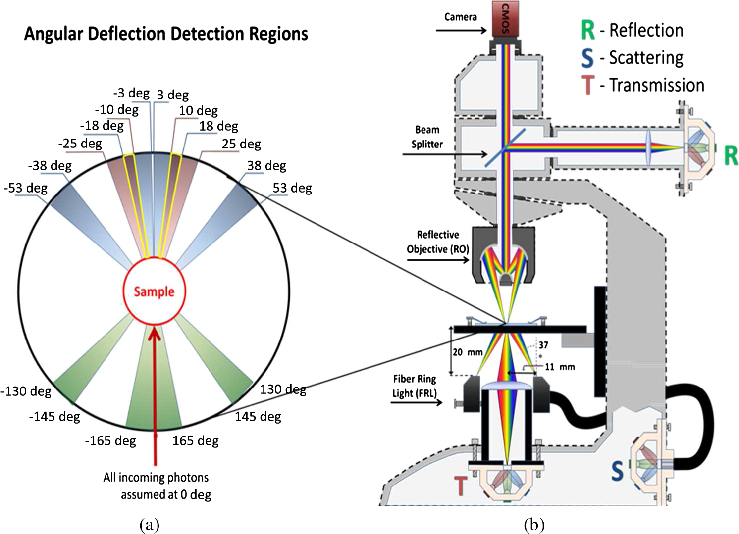

The camera used was a 5MPix ($2592\times 1944$) monochromatic CMOS camera (Guppy-503B, Allied Vision Technology, with a MT9P031 sensor from Micron/Aptina) with individual pixel size of $2.2\times 2.2\mu \text{m}$, each having a 12-bit pixel depth. In order for the broad spectral range to be imaged at the fixed image plane of the imaging chip, dispersion was minimized by using quartz lenses and a reflecting objective (Edmund Optics, NT58-421) with $15\times$ magnification and. 28 NA, giving an estimated point spread function (PSF) range of. 67 to 1.68 μm for the wavelength range used. The illumination to measure scattering was accomplished through a fiber-optic ring light (Edmund Optics, NT54-176) device (FRL) where the light emerges at the circumference of a circle situated at a certain distance below the sample. The fibers inside the ring are tilted inward so that the light field converges at the distance of the sample.

There are two important things to note regarding the ability of the system to collect light, and they are in regard to the reflecting objective and the FRL. The objective has a Cassegrainian type of telescope arrangement, where essentially a concave and a convex mirror work in conjunction to magnify the light. In this configuration, the convex mirror surface is located directly on the optical axis and thus blocks part of the light in all angular modes (see Fig. 1). Regarding the FRL, light emerges at a tilt angle of 37 deg to the normal from the circumference of a circle having a diameter of 22 mm. Therefore, changing the height of this source in relation to the sample will change the angle at which light impinges on the sample. This height was set at 20 mm during the experiment, which provided the detection sensitivity regions demonstrated in Fig. 1. These aspects, with regard to the objective and FRL, should be taken into account when analyzing the scattered light from malaria samples. There is an overlap of detection regions between transmission and scattering indicated with yellow lines. These can be adjusted to overlap less by moving the FRL in the vertical direction; however, this was not realized at the time the measurements were made.

The different angular modes complement each other providing essential information, but each also suffers some disadvantages. The transmittance mode yields good assessment of absorption properties but low contrast for transparent constituents. The reflectance mode provides an indirect measurement of the sample’s refractive index as well as the surface orientation and thus curvature of the RBCs while the high reflectance from the microscope sample slide provides a low contrast. Internal structural properties of the RBCs can be revealed in the scattering mode although the illumination efficiency is low. However, this can be improved by proper collimation of the ring light. In summary, the transmittance mode provides information of the chemical composition of the RBCs, reflectance is related to the outer shape, while scattering provides information about the internal organelles such as parasites. The concept of a multiangular mode system, sampling the scattering phase function at multiple intervals, was of key importance in the optical design in order to acquire the angularly and spectrally rich information from single scattering. This advantage becomes less significant when approaching the diffusing regime for thick or highly scattering samples where the information about the original direction of propagation is lost during the multiple scattering events. In single scattering, we are able to observe the internal structures with improved contrast arising from surfaces with different refractive indices. Increased contrast by single scattering has also been demonstrated from crystalline hemozoin at certain angles of backscattering.¹²

2.3.

Image Acquisition

The system was controlled from a PC using a custom-made program in LabVIEW™ (National Instruments, NI) where images were captured and saved in 16-bit unsigned integer images in TIFF format. For each illumination wavelength, a bright and a dark reference image was acquired, but, depending on which angular geometry was used, these recordings were done differently. For transmittance and reflectance measurements, the bright reference was an empty microscope slide placed in the object plane, whereas for scattering measurements an opal diffuser was used. Camera exposure times and gains were adjusted to give the highest intensities in the image without saturating the bright references. The dark reference images for transmittance and reflectance were taken by disconnecting the illumination current and using the same exposure times as for the bright references. For the scattering dark reference, the opal diffuser was simply removed and acquisition parameters for the scattering bright references were used. All acquisition parameters were set with the bright references, after which the sample was placed in the object plane and imaged for all three angular geometries. It was of importance to acquire all sample images for all geometries consecutively, keeping the sample in the same location in order to compare transmittance, reflectance, and scattering properties of single RBCs.

2.4.

Image Analysis

Once all images were taken and saved, they were analyzed using a customized algorithm in MatLab® (MathWorks). Initially, the background images were subtracted from all sample images. Then the normalization procedure was made differently for the three angular modes. For scattering, the dark reference image (${\mathrm{Im}}_D$) was subtracted from the sample (${\mathrm{Im}}_S$) and the bright (${\mathrm{Im}}_B$) reference images. Then the sample image was divided by the bright reference image to obtain the normalized image (${\mathrm{Im}}_{\text{Norm}}$) according to Eq. (1):

For reflectance and transmittance, an algorithm was written to automatically find the regions in the sample image where there were no RBCs. A two-dimensional (2-D) polynomial fit was applied with the intensity values in these regions; thus, a virtual bright reference image was extracted from the sample image and Eq. (1) was used. In this flat-field calibration, the intensity values given for each pixel were normalized with respect to the nearest empty region, which means the image is in effect not normalized to the microscope slide only, but to the regions free from RBCs. Normal human blood consists of 55% plasma (90% water and 10% proteins) and 45% cells,^12,23 which suggests that the normalization is made not only to the microscope slide but also to some plasma residue. Finally, to remove noise, a 2-D median filter was applied to the normalized images.

Following the normalization, the centers of all RBCs were manually selected in the entire image, since we did not have a trained algorithm to find them automatically. Once the spectral fingerprints of infected cells have been determined, this step can be automated. For each RBC, the spectrum for reflectance, scattering, and transmittance was extracted and concatenated into one vector having 39 elements ($3\text{geometries}\times 13\lambda$). Spectra for 453 RBCs were extracted and singular value decomposition (SVD) was used.³¹ SVD is a multivariate technique where the data are transformed into a new hyper-dimensional coordinate system where variance is maximized along each dimension representing a specific variable. From the transformation of the original data (${\mathbf{M}}_{n,\lambda }$, where $n$ represents a specific RBC out of a total number of $N$ RBCs, and $\lambda$ the wavelength), three arrays can be extracted, where base-spectra (${\mathbf{V}}_{\lambda ,m}$, where $m$ represents the spectral component), eigenvalues (${\mathbf{\Sigma }}_{m,m}$) and linear coefficients (${\mathbf{U}}_{n,m}$) represent the original data according to Eq. (2),

The base-spectra, also called loadings, are a new set of base functions of the original data, which are all orthogonal to each other. Because of the orthogonality between all vectors within $\mathbf{V}$, they represent the original data much more efficiently where the first column in this matrix represents the most significant spectral component, the second column the second most significant, and so on. Therefore, the first base-spectrum resembles the average of all original spectra for the RBCs over all wavelengths, naturally so since the average is the best summary of all data. $\mathbf{\Sigma }$ contains the eigenvalues for each eigenvector representing the importance of each eigenvector in relation to the others. This allows for removal of the eigenvectors that provide no additional contrast. $\mathbf{U}$, also called scores, contains the linear coefficients for each RBC explaining how much of each eigenvector is required in order to recreate the original spectrum for that RBC. With this information, we can reduce our original data to represent the significant contrast with only a few base-spectra rather than all contained in the original data by the removal of insignificant variables for the desired contrast. Adding more dimensions will not provide any additional contrast but only increases the noise and reduces the potential contrast of the outcome. In our case, each eigenvector represents one LED for a specific angular geometry, thus giving us 39 PCs (principal components). Not all illumination bands gave a strong contrast between the cells, and this became evident using SVD.

Hierarchical clustering and dendrogram representation³² were applied to summarize the interdistance of the SVD scores to see if there were any discrete clusters of data points in the new coordinate system and how related these were. The number of dimensions from the SVD analysis was truncated to 3; thus, the algorithm clustered all 453 data points into an equal number of clusters. The number of clusters was chosen to equal the number of dimensions because we essentially select to observe the data with a reduced number of observations (dimensions).³² If the number of clusters is greater, the observations would no longer be linearly independent, and we would have to account for factors that are not observed from the reduced data. From each data point, a line is drawn to all the other data points in this new Euclidian space, and the length determines how related they are. The shorter the line, the greater the chances that two points belong to the same cluster or that they are from two closely related clusters. This information is presented in a dendrogram, which gives an overview of how close the clusters are to each other in the Euclidean space. From this dendrogram, the RBC coordinates belonging to each group can be marked in the original image and the average spectra for all clusters can be extracted, plotted, and compared with each other.

3.1.

True-Color Representation of Single RBCs

Measurements were taken at the following wavelengths: 380, 405, 430, 480, 525, 600, 630, 660, 700, 760, 810, 850, and 935 nm in transmittance, reflectance, and scattering. Using MatLab, true-color representations of the sample were constructed by combining the normalized images taken at 630 nm (red), 525 nm (green), and 480 nm (blue) (Fig. 2). Thus the images appear as if one would manually observe them through the microscope binocular under white light illumination. Figure 2 shows the same region of the sample in all three angular modes. Since all measurements for the three angular modes were taken without moving the sample, one can compare the three modes in each pixel. However, the effective pixel-size is far below the diffraction limit set by the imaging system. This means one pixel is affected by a number of near-lying pixels and can therefore not be considered individually. However, evaluating the RBC as a whole, one can argue that pixels from different parts of the RBC play different roles in the differentiation between healthy and infected cells. Therefore malaria criteria should be applied on a pixel level but evaluated on a whole cell level; in Fig. 2 we can clearly see the RBCs to be distinctly separated. The following images show a cropped out region from the original image to better show the appearance of individual RBCs; however, all analysis was made on the full image containing 453 RBCs. It becomes evident from these true-color representations that there are significant differences between RBCs in all three geometries, but for different reasons.

Fig. 2

(a) to (c) True-color representation of the images taken for the three angular modes where spectral differences are seen in all, but to different degrees. 2(a) (reflection) shows the decrease in reflection in some RBCs where the central region appears darker, which can be attributed to the typical doughnut-shape of RBCs. 2(b) (scattering) shows the largest contrast between the RBCs. 2(c) (transmission) shows some RBCs absorbing more light than others in a centralized region, thus appearing as darker spots. The central red dot is most clearly visible in the scattering geometry.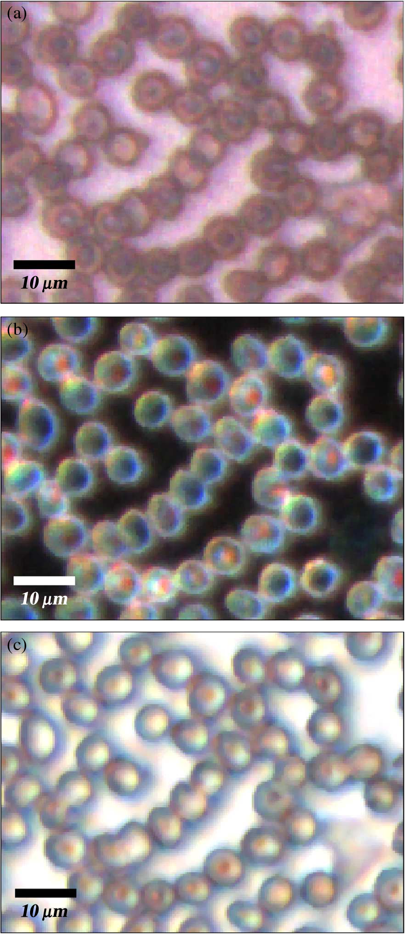

In Fig. 2(a) (reflection) we can see the expected red color of the RBCs, but there is a clear distinction between the cells. Some cells appear slightly brownish whereas others appear redder. The contrast is most evident in Fig. 2(b) (scattering) where we can clearly see the RBCs seemingly having an internal structure. Those without internal structure appear to have hollow centers whereas those having something concrete inside scatter significantly. In the acquisition for scattering, the FRL is aligned so that in the absence of a sample, the majority of the light passes outside the aperture of the objective. Thus, when there is something in the sample plane deflecting the light from its original path into the aperture of the objective, a signal is measured from what we define as zero, being the dark reference. In Fig. 2(c) (transmission) the light passes through the RBCs, and we can observe a reduced transmittance from some cells compared with others. There is an apparent darker region in the center of some RBCs, which seems to slightly change from cell to cell. One reason why the cells appear white rather than red is because they have been normalized to the regions free from cells. These regions contain blood plasma, which has similar spectral characteristics as haemoglobin,²³ and thus the RBCs appear white rather than red. In this aspect, the transmission sample would not appear as it does in Fig. 2(c) to the human eye. What is interesting is that Fig. 2(a) is also normalized to the region free from RBCs, but there is a larger contrast due to the scattering properties of RBCs where the back-scattered light is significantly stronger when the light is incident at an angle to the normal of the RBC surface,²⁴ which, according to Fig. 1, cover the photons that are deflected at angles between 35 deg to 50 deg and 0 deg to 15 deg from their incidence. We also see that the angular sensitivity regions for transmission lie close to the optical axis as these photons are not deflected far from it. This is another contributing reason to why higher intensities can be measured from the cells compared with the white reference (empty slide) as the forward-scattering property of individual RBCs tends to increase the intensity when the angle of the incident light approaches the plane perpendicular to the optical axis.²⁴

Comparing all angular modes, we can see that the invisible characteristics in transmission become clearly visible in scattering. In general we see that the differences of the cells in each angular mode correlate well between the angular modes; the same RBC having a brown spot in Fig. 2(c) (transmission), appears browner in Fig. 2(a) (reflection), and has a red spot in the center of Fig. 2(b) (scattering). From the three images in Fig. 2, we can draw a conclusion that some RBCs have some sort of internal structure, which will be discussed further below. According to the life-cycle of the Plasmodium falciparum parasite, where during its trophozoite stage it enters the RBCs and grows within, we can expect to see the infected cells having some sort of internal structure.¹¹ We keep this in mind as we continue to apply statistical methods for all RBCs in all geometries and spectral bands.

3.2.

Singular-Value Decomposition and Hierarchical Clustering

Before any further analysis was made, the spectra had to be collected from the RBCs. This was done by cropping out a region with a three-pixel radius from the center of the RBC, over which an average intensity was acquired at each spectral band. Thus a spectrum for every RBC in each geometry was extracted at a spectral resolution of 13 bands from 380 to 935 nm. In order to perform the SVD analysis, we had to concatenate the spectra from the three different geometries into one for each RBC, which is seen in Fig. 3(a). In this plot we can see the general trend of how not only the spectral characteristics change throughout the three angular modes, but also the variance between the blood cells. In Fig. 3(b) we see the extracted eigenvalues, which are the diagonal elements of $\mathrm{\Sigma }$, once SVD has been applied. To determine where to truncate our data, we had to study the relevance of the signal of each $\mathrm{\Sigma }$ in comparison to what we define as noise or, rather, irrelevant information. The noise level was chosen from the apparent plateau in Fig. 3(b), where a black line is interpolated through the plateau. Based on this noise level, ${\mathrm{\Sigma }}_{1,1}$ gives a signal-to-noise ratio of approx. 6:1, ${\mathrm{\Sigma }}_{2,2}$ approx. 3:1 and ${\mathrm{\Sigma }}_{3,3}$ slightly less than 2:1. We decided that this was the lowest we would go before adding another PC did not provide additional relevant information. Therefore, the first three $\mathrm{\Sigma }$ were used as indicated by the three red circles in Fig. 3(b). In Fig. 3(c) the first three base-spectra are plotted in different colors, and they are separated into their respective angular geometry. Comparing Fig. 3(a) and 3(c), we see that from the first three base-spectra we can more or less describe all the original spectra for the RBCs in different linear combinations. How much of each eigenvector we use is indicated in $\mathbf{U}$ for each RBC, and we recreate the original spectra from the reduced set of coordinates according to Eq. (2),

Fig. 3

(a) shows the collection of spectra from all RBCs concatenated between the three angular modes. The rather large variance becomes evident. Figure 3(b) shows the eigenvalues for each PC where the first three are considered to be most relevant as their SNR is 2:1 or higher. The noise level is indicated with a black line drawn through the apparent plateau. The y-scale is logarithmic. Figure 3(c) shows the first three base-spectra for all PCs, and it is evident that the original data can be represented quite well with these curves. The spectra have been divided up in the angular modes.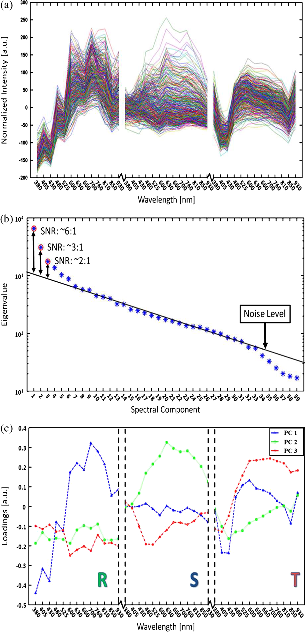

From the new coordinate system, the Euclidean distances between all points were calculated in order to determine which cluster they belong to. The relation between these three clusters is shown in the dendrogram in Fig. 4. On the $y$-axis, the values represent the distance in the Euclidian space, which was previously transformed with the SVD analysis; thus the values carry no units. Note that the color coding is not related to Fig. 3 but rather to the spectra in Fig. 5. Overall we can see that clusters 1 and 2 are closer related to each other than cluster 3. From the 453 RBCs examined, 9 fell into cluster 1, 118 into cluster 2, and 326 into cluster 3. Also evident in the figure are several subclusters. We chose three clusters, but there is of course a possibility that there are more variables that differentiate RBCs. However, the three clusters seem to be significantly separated to motivate a comparison of them, and this should become more evident when examining their spectral characteristics in the following section.

Fig. 4

Dendrogram representation of all the RBCs and their relation according to the reduced variables from the SVD analysis. The color coding is kept for the next section where the spectra are shown for each cluster. The y-axis represents the Euclidean distance in the newly formed coordinate system and therefore carries no units. In cluster 1 there are nine RBCs; in cluster 2 there are 118 RBCs; and in cluster 3 there are 326 RBCs.

Fig. 5

(a) to (c) Average spectra for the three clusters in the three angular modes. In all spectra we see contrast to some extent between the three clusters. 5(a) (reflectance) shows a progression from cluster 1 to cluster 3 of an increase in reflectance. 5(b) (scattering) exhibits the strongest contrast where the progression of increased scattering goes from cluster 3 to cluster 1. 5(c) (transmission) shows an increase in absorption from cluster 3 to cluster 1, which we can understand from 5(a) where we saw a decrease in reflectance in a similar fashion.

3.3.

Individual RBC Spectra in all Angular Modes

Tracing back the color space coordinates for the data points in the clusters, we took the average spectrum for each cluster and plotted them separately for each angular geometry seen in Fig. 5. In all spectra we can see some differences between the different clusters, but some promote the contrast more than others. What becomes clear is the progression as we observe all three clusters. Cluster 3 has by far more RBCs than the other two, followed by cluster 2 and, finally, very few RBCs in cluster 1. Remembering the life cycle of the malaria parasite, we note that when it enters the RBC in its trophozoite stage it consumes haemoglobin. Then it makes sense that we can see a progression as RBCs would naturally be in different stages of infection; the longer the parasite has been occupying the RBC, the more its spectral characteristics would differ from a healthy RBC. In Fig. 5(a) (reflection), we would also expect to see a decrease in reflection due to the high absorption at the characteristic Soret absorption band of haemoglobin at 405 nm, but it seems to have shifted to around 430 nm. This can partially be explained by the scattering characteristics of RBCs, which heavily depend on the shape and orientation of the cell as well as the angle of the incident light. There is a progression of increased reflectance moving from cluster 1 to cluster 3 as well as a general increase of reflectance from 480 up through 930 nm. In Fig. 5(b) (scattering), we see the largest contrast where all three clusters differ significantly from 480 nm and above, where cluster 1 and 2 seem to peak around 630 nm. It does make sense that the scattering geometry gives the strongest contrast because not only the parasite, but also the hemozoin that it expels, has structure providing contrast with regard to a healthy cell containing only haemoglobin.²⁷ The changing of spectral characteristics is most apparent in scattering going from cluster 1 to cluster 3, where scattering significantly increases for all wavelengths above 430 nm. In Fig. 5(c) (transmission), we see the characteristic Soret absorption of haemoglobin clearly at 405 nm, which appears to be at more or less the same level in all clusters, with perhaps a slight increase in absorption for clusters 1 and 2. What is more apparent in transmission is the increased absorption over the spectral region 480 to 810 nm as we move toward cluster 1 from cluster 3. The increased absorption can be paralleled with the decreased reflectance comparing the clusters.

3.4.

Mapping of Cluster Classifications onto RBCs

Once the three clusters were determined, the respective coordinates were marked on the true-color images to get a visual perception of how the different RBCs would appear to the human eye if observed directly through the binoculars of a microscope. Figure 6 is the same as Fig. 2, but having all RBCs marked with their respective cluster where cluster 1 is represented with a blue triangle, cluster 2 with a green square, and cluster 3 with a red circle. Note that some RBCs are not marked at all since they were not counted in the original list for reasons such as lying too close to a border or having an odd shape. Note also that the analysis was applied to the full image where Figs. 2 and 6 only shows a small region for better visibility.

Fig. 6

(a) to (c) From the three different clusters marked in this true-color image, we see significant distinctions in all angular modes, where the largest is again seen in scattering. 6(a) (reflectance) only shows a small, but still significant variance between the different clusters. It is more evident in 6(b) (scattering) as well as 6(c) (transmission). Cluster 1 is clearly distinct from cluster 3 in 6(b), which was already evident in Fig. 5(b). Some of the markings are not centered, which is due to the initial selection not being exactly in the middle of the RBC, but due to the cropped out region being significantly smaller than the RBC, it should not play a significant role.

In Fig. 6(a) (reflection), we see a distinct contrast difference between the clusters, but it is not as clear as for the other two other angular modes. This we can understand from the results in Fig. 5(a), where the reflectance spectra do not show large contrast between the clusters. However, we can see significant differences between the general appearances of the RBCs belonging to the different clusters. RBCs belonging to clusters 1 and 2 seem to progressively get darker and browner compared to the RBCs in cluster 3. Figure 6(b) (scattering) provides the largest contrast, as expected from the spectra in Fig. 5(b). The red spots seen in the RBC centers are clearly visible in clusters 1 and 2 and clearly not in cluster 3. Comparing cluster 1 with cluster 2, there appears to be a slight difference in visibility of the red spot. The previously discussed progression of the spectra is most visible in Fig. 6(b) for scattering, where all RBCs belonging to cluster 1 have the brightest red spots in the center. There is also a number of RBCs belonging to cluster 2 having the bright spot but not as bright as the ones from cluster 1. All RBCs belonging to cluster 3 are lacking a red spot in the middle. From Fig. 6(c) (transmission), we see there are differences between the three clusters where there is an apparent brown spot in the center of the RBCs belonging to cluster 1 and 2, and not in cluster 3. Between cluster 1 and 2, we again see the slight difference in visibility of the spot in the center. The fact that the spot in the middle is brown in transmission and reflection and red in scattering is due to the different normalization procedure for the acquisition modes previously discussed.

3.5.

Malaria Expert Evaluation

The blood smear was independently analyzed visually by Jeremie T. Zoueu, who has considerable experience in malaria evaluation. For all studied RBCs, he had to decide whether the RBC was infected or healthy by visual examination as each RBC was individually presented on a computer screen as shown in Fig. 2. If he was uncertain to determine an infection he could also indicate that (Fig. 7 shows a chart with the corresponding classification). The results are presented cluster by cluster where the percentage represents how many of the RBCs in that cluster belong to each expert classification. Cluster 1 has 9 RBCs, out of which 22.2% are indicated as healthy, 44.5% are indicated as infected, and 33.3% uncertain. Cluster 2 has 118 RBCs, out of which 70.3% are indicated as healthy, 5.1% infected, and 24.6% uncertain. Cluster 3 has 326 RBCs, out of which 93.8% are indicated as healthy, 1.5%, infected and 4.7% uncertain. This gives a total of 391 healthy and 15 infected RBCs with the certainty of the expert; thus, over the entire sample, our expert confirms that 3.3% are infected. Malaria parasiteamia ranges depending on the severity of the infection as well as the age of the patient. The rate found from a study in 1995 was 1.6% for children aged 1 to 4 and 5.5% for patients of 15 years and up.³³ From this we can say that our results are acceptable. However, a proper procedure of first using our microscope and then directly after staining the sample and applying a conventional counting method was not performed. For this reason we cannot give any value of specificity and sensitivity but rather conclude that our method gives promising results in good agreement with an expert in the field having used conventional methods. We can also infer from the chart that the percentage of infected cells decreases as well as the number of healthy cells increases from cluster 1 to 3. Although the number of RBCs in cluster 1 is significantly lower than cluster three, the majority of them are infected. This is a strong indication that our routine can identify malaria-infected blood cells without the use of staining.

Fig. 7

A chart showing the distribution of healthy and infected cells for the different clusters analyzed by our malaria expert. In each cluster there is also a column indicating how many blood cells the expert could not properly distinguish. The trend becomes obvious as the number of infected cells strongly decreases as we go from cluster 1 to 3. Similarly, the number of healthy cells increases from cluster 1 to 3.