1.

Introduction

Volumetric optical coherence tomography (OCT) is rapidly emerging as a dominant diagnostic imaging modality in ophthalmology. High resolution volume scans in clinical OCT imaging sessions can last up to several seconds, requiring the subject being imaged to stay perfectly still, fixating gaze at a single point. Even small movement of the subject can lead to undesired motion artifacts in the resulting acquired images. Eye tracking hardware can also be used to minimize motion artifacts, but this in turn adds to the cost and complexity of the system. This is the reason many researchers are working on methods to reduce the overall OCT scan acquisition time.

Efforts to reduce the overall scan time predominantly concentrate on increasing the speed of the hardware of the OCT system.¹ The net increase in speed from this approach is limited because the system sensitivity (and image quality) is inversely related to the acquisition rate.^2,3 The optical power at the sample for ophthalmic applications cannot be arbitrarily increased because the American National Standards Institute (ANSI) sets strict limits on the maximum permissible optical exposure in the eye.

Another method of increasing the volumetric data rate is to change the scanning protocol. The traditional raster scan approach⁴ is often wasteful for objects such as the optic nerve head (ONH) because peripheral lines do not intersect the features of interest. Recent advances from information theory, known as compressed sensing (CS),^5–7 have allowed researchers to decrease the overall OCT scan time by reducing the number of acquired image samples without significant degradations in image quality^8–10 in terms of mean squared error (MSE) and Structural SIMilarity index (SSIM).¹¹ These methods, combined with fast OCT hardware, are based on pseudo-randomly acquiring small subsets of the image volume and then using an efficient CS-based recovery scheme from subcritical samples, hereafter simply referred to as ‘interpolation,’ to reconstruct the image samples that were not acquired.

Radial OCT image acquisition^12–14,15 has been proposed as a method to augment the regular raster-scan pattern. Radial scanning inherently collects a denser distribution of image samples closer to the center of the image, and a sparser distribution of samples in the peripheral regions of the image. In certain imaging applications, like imaging of the optic nerve head, this is the preferred scan pattern since each acquired B-scan contains a cross-sectional image of the optic cup. Volumetric reconstruction of the ONH is particularly important for emerging clinical imaging applications investigating correlations of morphology of ONH and susceptibility of glaucoma.¹⁵ To display and render the radially acquired samples, the data must be resampled to a regular Cartesian grid where the subsequent visualization, volumetric rendering and morphometric analysis can be performed. Resampling the data to a Cartesian grid can be achieved through a simple radial to Cartesian coordinate transformation. However, accurate interpolation of image samples collected from a radial grid is a nontrivial task.^16–18 The most common method to interpolate radially sampled data is to employ radial basis functions. While these methods shows promise, they lose some of their advantages when there are large gaps present in the data, which is typical in radial sampling away from the center.

In this work we describe a novel random-radial sampling method and a novel technique to reconstruct data acquired by this sampling scheme to interpolate volumetric OCT image data. In the context of this work, a random-radial scan pattern refers to a scan pattern consisting of radial B-scans, with a random angular separation between each subsequent B-scan. On one hand, this technique leverages the concepts of sparse sampling by acquiring randomly spaced angular measurements, while on the other hand it acquires image samples that can be directly used for clinical measurements of the ONH such as retinal thickness.¹⁴ In accordance with the principles of CS, the interpolation on the collected data is performed in a transform domain, which matches the symmetry of the acquired volume. We demonstrate the proof-of-concept of radial-CS by analyzing three recovered human ONH datasets and investigating the resulting morphometric measurements for different percentages of missing data. The image quality is compared based on standard morphometric analysis used in the clinic.

2.

Methods

In this section, we describe the proposed procedure for volumetric OCT imaging using sparse radial samples. Volume acquisition is performed by randomly spaced radial B-scans. In the context of this work, random-radial B-scans refer to scans where the angle of a subsequent B-scan, relative to the previous B-scan, is drawn from a random distribution. Radial B-scan spokes, each consisting of a fixed number of A-scans, are acquired at a random angular spacing within a range defining the maximum and minimum step size. The sparseness of the acquisition is determined by the maximum allowable angular step size. In order to interpolate the data in the regions which have not been acquired, a mapping is first implemented which places the acquired radial spoke B-scan images in a three-dimensional (3-D) Cartesian system. This mapping converts ($r$, $\theta$, $z$) coordinates to ($x$, $y$, $z$) coordinates, where $x=\theta$ and $y=r$. Essentially, this is the stacking of each radial B-scan in a 3-D Cartesian grid where the placement in the horizontal direction is based on the angle of the radial scan, as shown in Fig. 1(a) and 1(b). The missing radial scans then become equivalent to missing vertical Cartesian raster scans in the ($r$, $\theta$, $z$) space.

Fig. 1

A schematic outlining the proposed procedure. (a) Acquisition of several randomly spaced radial B-Scans. (b) Stacked radial B-scans in the ($r$, $\theta$) spaces. (c) Interpolated data in the ($r$, $\theta$)space. (d) Data from (c) is mapped back to the Cartesian grid to produce and interpolated radial image.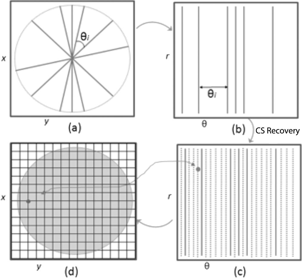

Reconstruction of the missing data is now performed by the CS-based interpolation method described in Ref. 8. Briefly, we let $f$ denote the full 3-D tissue image, $R$ to be the 3-D restriction mask that restricts the image samples actually acquired, $M$ to be the measurement basis and $y$ to be the image samples actually acquired. Given this, the sparse image acquisition problem can be formulated as $y=RMf+n$ where $n$ is the noise in the collected data. If $S$ is some transform domain that offers good compressibility of $f$, and $x=Sf$ are the transform coefficients of $f$ then $f$ can be exactly reconstructed by $f=S^{H}x$, where $S^H$ is the synthesis of $S$. Instead of directly recovering the image $f$, we find a set of coefficients $\tilde{x}$ so that $\tilde{f}=S^H\tilde{x}$ is a good approximation of $f$. The approximating coefficients $\tilde{x}$ are found by solving the following constrained optimization problem:

Stated simply, we are looking for a solution that is sparse (small $l_1$-norm) and simultaneously has a faithful representation of the collected data (small $l_2$-norm between the observed data and synthesized coefficients). Results of Ref. 6 show that if $x$ is sufficiently sparse, then the solution to Eq. (1) is exact, up to the noise level $ϵ$, with overwhelming probability. The constrained optimization problem presented in Eq. (1) can be solved with Iterative Soft-Thresholding solver, described in Ref. 19.

Following the interpolation step [Fig. 1(c)], the vertically aligned B-scans in the 3-D Cartesian volume represent the radial scans that were mapped to lie in this coordinate system. To map the interpolated data back to the physical 3-D Cartesian volume, we apply the inverse of the mapping that placed the radial scans in the ($r$, $\theta$, $z$) space ($x=r\cos \theta$, $y=r\sin \theta$, $z=z$). The result is that the 3-D image voxels of the whole field of view have now been reconstructed in their physically corresponding positions i.e., the missing data in between the acquired radial scans has been filled in, and in a way such that the reconstructed samples are located on the 3-D Cartesian grid (the standard image storage format) overlaid in the field of view.

The construction of the radial sampling pattern can be done by choosing the first radial scan to be horizontal, and thereafter incrementing the radial angle in angle increments that are drawn from some random distribution, with some upper limit on maximum allowable angle between any two adjacent scans. For example, one way of choosing the angle increment would be to draw it from the uniform distribution over $[0,\pi /18]$ i.e., the maximum angle increment is 10 deg. This maximum allowable angle is chosen depending on the size of the smallest feature we may want to resolve in the image. This is a major advantage of the proposed new scan pattern for OCT as the information of interest, the optic nerve head, or other features such as the morphology of the fovea or the macula, can be position to be in the center where they are densely sampled. The angle increment between B-scans can be made larger and this would sacrifice the resolvability of features in the periphery of the field of view but retain high fidelity in the center.

It is important to note that compressive sampling, as introduced by Ref. 7, under certain assumptions, guarantees exact signal reconstruction from multiple random projections of the signal being observed. With the OCT image acquisition setup proposed in this work, we are not acquiring random projections, but instead acquiring a random subset of the image in the pixel domain. This requires a reformulation of the sensing matrix to make our formulation adhere to the principles of compressive sampling. Specifically, the sensing matrix is factored into ${RMS}^H$, where $R$ models our proposed random sampling pattern in the ($r$, $\theta$, $z$) space, $M$ is the Dirac measurement basis, and $S^H$ is the synthesis of the wavelet transform. In Sec. 2.1 we demonstrate that OCT images have a relatively sparse representation in the wavelet domain.

The other necessary condition to achieve good CS-based signal reconstruction is that the mutual coherence, $\mu$, between the sensing and representation bases must be small.²⁰ The smaller the coherence is between the sensing and representation bases, the fewer image samples are required to reconstruct the image. Essentially, $\mu$ is the largest correlation between any two atoms of the sensing and sparsifying transforms. Figure 2 shows several wavelet atoms in the physical (Dirac) domain, plotted at different scales. The figure is generated by applying a wavelet analysis operator to a zero matrix, inserting a unity at several locations corresponding to different scales, and applying a synthesis operator to visualize wavelet atoms in the physical domain. At least qualitatively, we can see the large spread of wavelets, and hence their incoherence in the Dirac basis. Combining this with the fact that OCT images appear to be compressible in the wavelet domain, this makes our formulation commensurate with the ideas of compressive sampling. There exist many works, Refs. 21 and 22 to name a few, that have employed similar ideas to reconstruct images from missing information in the pixel domain with high fidelity.

Fig. 2

Wavelet atoms shown at different scales in the physical domain. Scale 1 corresponds to the coarsest scale, while scale 5 corresponds to the finest scale. The dashed lines represent the approximate windows of support for each wavelet atom.

2.1.

Choice of Sparsifying Transform

Successful CS-based signal recovery largely depends on the choice of the sparsifying transform $S$, as defined in Eq. (1). One of the key factors in choosing a proper sparsifying transform is the transform’s ability to efficiently represent the data—that is, most of the signal’s energy should be captured by only a few transform’s coefficients. We investigated three transforms’, Daubechies wavelets $S_w$, Curvelets $S_c$,^23,24 and Surfacelets $S_s$,²⁵ abilities of efficiently capturing the energy of our OCT volume. These three transforms are commonly used in CS-based applications to reconstruct signals from incomplete measurements. We investigated this ability by computing the transform’s coefficients $x_i$ by applying the analysis operator $S_i$ to the model OCT volume $f$, shown in Fig. 3. That is, $x_i=S_{i}f$, where $i\in (w,c,s)$. Figure 4(a) shows the normalized coefficients $x_i$ plotted in magnitude-decreasing order. We also computed the mean squared error (MSE), defined by ${\Vert f-\hat{f}\Vert }_2/{\Vert f\Vert }_2$, of partial reconstructions $\hat{f}$ by applying the synthesis operator $S_i^H$ to a set of restricted coefficients $x_{i,\eta }$. That is, ${\hat{f}}_i=S_i^H{x}_{i,\eta }$, where $x_{i,\eta }$ retains only the $\eta$ largest coefficients, and thresholds the rest to 0. Figure 4(b) shows the MSE, as a function of the number of coefficients $\eta$ used in the reconstruction. Since Wavelet coefficients have the fastest decay rate and the smallest MSE of partial reconstructions, we can say that relative to curvelets and surfacelets, the OCT volume is compressible under Wavelets, and thus we use the Wavelet transform in all further computations.

Fig. 3

Extracted en-face slices from Volume1, recovered with 200, 100, and 60 random-radial scans. Images in the first column show extracted B-scans form the fully sampled volume1. Images in columns 2, 4 and 6 show B-scans extracted from data volumes sampled with 200, 100, and 60 random radial B-scans, respectively. Images in columns 3, 5, and 7 show extracted B-scans from volumes recovered with 200, 100, and 60 random radial B-scans, respectively.

Fig. 4

(a) Normalized relative decay rates of Wavelet, Curvelet and Surfacelet coefficients of stacked radial B-scans in ($r$, $\theta$, $z$) space, sorted in decreasing order. (b) Mean squared error of reconstruction of the model volume in ($r$, $\theta$, $z$) space, shown in Fig. 3 from a partial set of transform’s coefficients.

3.

Results

Model data to investigate the performance of CS-OCT was acquired by raster-scanning the ONH of three healthy subjects using a custom built Michelson interferometer based Fourier-domain OCT system. We employed X-Y galvanometer mounted mirrors (6210H, Cambridge Technology Inc., Lexington, Masachusetts) to scan the beam across the area of interest. The light source was a commercial swept-source laser with an operating wavelength of 1060 nm from Axsun Technologies (Billerica, Masachusetts) with an effective 3 dB bandwidth of 61.5 nm, corresponding to an axial resolution of $l_c=6\mu \text{m}$ in tissue. The optical system used a standard fiber coupler Michelson interferometer topology and the sample arm optics delivered a spot size of 1.3 mm at the cornea and 17 μm at the retina (assuming the axial eye length is 25 mm). For details on the experimental setup we refer the reader to Ref. 9. For all three acquired volumes the B-scans consisted of $1024\times 400(\mathrm{axial}\times \text{lateral})$ pixels. The en-face area covered by the scan for the first subject was 4.4 by $4.4{\mathrm{mm}}^2$, while the en-face scan area for both subjects 2 and 3 was 7.2 by $7.2{\mathrm{mm}}^2$. We will subsequently refer to the thee acquired volumes as volume1, volume2 and volume3. Volume1 is a comparatively small scan, nominally centred at the ONH. Volume2 is a larger scan which includes the ONH and macula in the periphery of the image. Volume3 is a scan of the same size as volume2, and is nominally centred on the ONH. Representative B-scans from the three acquired volumes are shown in the first columns of Figs. 3, 5, and 6. Note that the scans were approximately centred at the ONH for volumes1 and 3, while for volume2, the scan was purposefully off-centre from the ONH.

Fig. 5

Extracted en-face slices from Volume2, recovered with 200, 100, and 60 random-radial scans. Images in the first column show extracted B-scans form the fully sampled volume2. Images in columns 2, 4 and 6 show B-scans extracted from data volumes sampled with 200, 100 and 60 random radial B-scans, respectively. Images in columns 3, 5, and 7 show extracted B-scans from volumes recovered with 200, 100, and 60 random radial B-scans, respectively.

Fig. 6

Extracted en-face slices from volume3, recovered with 200, 100, and 60 random-radial scans. Images in the first column show extracted B-scans form the fully sampled Volume3. Images in columns 2, 4, and 6 show B-scans extracted from data volumes sampled with 200, 100, and 60 random radial B-scans, respectively. Images in columns 3, 5 and 7 show extracted B-scans from volumes recovered with 200, 100, and 60 random radial B-scans, respectively.

To simulate the data as it would appear if we were to acquire it with the proposed sampling pattern, we generated three different random-radial sampling masks each consisting of $n=200$, $n=100$ and $n=60$ radial B-scans. Correspondingly, each level of subsampling comprises 61.5%, 80.9%, and 88.3% missing data. We take the first radial B-scan to lie on the horizontal axis, and each subsequent radial B-scan is incremented by a random angle, drawn from a uniform distribution over (0, $\pi /n$). With this type of construction the maximal angular increment is guaranteed to be ${\theta }_{\max }\le 2\pi /n$.

After applying the particular radial subsampling masks to the full volume, we recovered the missing data by the procedure detailed in the previous section. To interpolate the sparse samples in ($r$, $\theta$, $z$) space we employed the IST solver with 6 inner and 40 outer loop iterations. Total run-time for the interpolation algorithm with these parameters was approximately 2 h on a machine with an Intel i7 CPU running at 2.67 GHz and 20 GBs of memory. For details on how the total computational time of the recovery algorithm varies as a function of the number of iterations, we refer the reader to Ref. 10. We note that the implementation of the recovery algorithm, as implemented in Ref. 10 and used in our work, is implemented in Matlab. Since the recovery algorithm consists of matrix-vector multiplications and analysis/synthesis wavelet transforms, we anticipate that a significant reduction in scan time can be achieved by implementing it in a combination of C/C++ and utilization of GPU technology.

The results of the interpolation procedure for the three different volumes are shown in Figs. 3, 5, and 6. The top panel shows a typical en-face slice from the data volume. The colored lines show locations of six extracted B-scans. The left-most column shows the extracted B-scans from the original raster-acquired volume. The subsequent images show the corresponding B-scans as they appear in the data volumes and the resulting interpolated volumes. The mean squared errors of the resulting reconstructions from 200, 100, and 60 radial scans from each volume is reported in Table 1. In the next section we show that the quality of the reconstructed images remains adequate to make anatomically meaningful measurements, such as Total Retinal and Nerve Fiber Layer thickness accurate to within the intrinsic axial resolution of the OCT system used in this report.

Table 1

Mean squared error (MSE) values of the reconstructed volumes for different levels of subsampling.

3.1.

Validation

To validate the quality of the CS-based reconstruction algorithm for interpolating subsampled volumetric OCT images, we computed and compared for each volume the nerve fiber layer (NFL) thickness, total retinal (TR) thickness, and cup-to-disc ratio ($c/d$). For these measurements, we segmented the inner limiting membrane (ILM), the boundary between the NFL and inner plexiform layer (NFL-IPL boundary), Bruch’s Membrane (BM), and Bruch’s membrane opening (BMO). A 3-D graph-theoretic algorithm was used to automatically segment the ILM, NFL-IPL boundary, and BM.^26,27 In this method, a weighted geometric graph is constructed such that the nodes correspond to the voxels in the volume and arcs are created based on geometrical proximity, a smoothness parameter, and minimum and maximum distances between the surfaces. The target surfaces are segmented by computing a minimum closed set in this graph by a minimum s-t cut in a derived arc-weighted digraph. We used the MaxFlow Software²⁸ (v3.02) to compute the minimum cut. The cost function used here was intensity gradient in the axial direction. Thus the algorithm found the ILM, NFL-IPL boundary, and BM as the optimal surfaces given the intensity gradient, smoothness restriction, and inter-surface distance restriction.

The NFL-IPL boundary had lower contrast compared to the ILM and BM, and a trained human delineator manually corrected the NFL-IPL boundary segmentation in the regions where the automatic algorithm showed inaccuracies. To avoid bias, the delineator examined and corrected each volume separately. The BMO was also segmented manually.

The NFL thickness was defined and measured as the axial distance between the ILM and the NFL-IPL boundary. The total retinal thickness was defined and measured as the axial distance between the ILM and BM. The NFL and TR thickness maps for each of the recovered volumes are shown in Figs. 7 and 8, respectively. Note that in the thickness calculation, we excluded the regions where the BM and NFL are not visible. These regions are below the ONH, and in the case of volume2, the region below the fovea.

Fig. 7

Computed nerve fiber layer (NFL) thickness, shown in μm, on each of the three volumes (first column), and the NFL thickness computed from volumes reconstructed from 200 (2nd column), 100 (3rd column) and 60 (4th column) radial scans. The regions within the BMO and in the macula are masked white because NFL and BM are not defined in these areas.

Fig. 8

Computed total retinal thickness (TR) thickness, shown in μm, on each of the three volumes (first column), and the TR thickness computed from volumes reconstructed from 200 (2nd column), 100 (3rd column) and 60 (4th column) radial scans. The regions within the BMO and below the macula are masked white.

To localize the changes in thickness measurements, we plotted the differences in thickness between the fully sampled and the recovered volumes. The differences in NFL and TR thickness are shown in Figs. 9 and 10, respectively. We note that the greatest differences in thickness occur in the peripheral regions of the image, which are predominantly visible in volume2 and volume3 (Fig. 9 rows 2 and 3). To quantify the obtained thickness measurements we averaged the changes in NFL and TR thickness for each of the reconstructed volumes. These changes are reported in Table 2. We observed that the greatest change (7.9 μm) in computed TR thickness occurred in the reconstruction of volume3 from 60 radial B-scans. The greatest change in computed NFL thickness occurred in the same volume, and was 5.9 μm. Both of these changes are on the order of the intrinsic axial resolution ($l_c=6\mu \text{m}$) of the OCT system.

Fig. 9

The differences in nerve fiber layer (NFL) thickness, shown in μm, between the NFL thickness computed on the fully sampled volumes and the NFL thickness computed on volumes that were reconstructed from 200 (first column), 100 (second column) and 60 (third column) radial scans. $l_c=6\mu \text{m}$.

Fig. 10

The differences in total retinal (TR) thickness, shown in μm, between the TR thickness computed on the fully sampled volumes and the TR thickness computed on volumes that were reconstructed from 200 (first column), 100 (second column) and 60 (third column) radial scans. 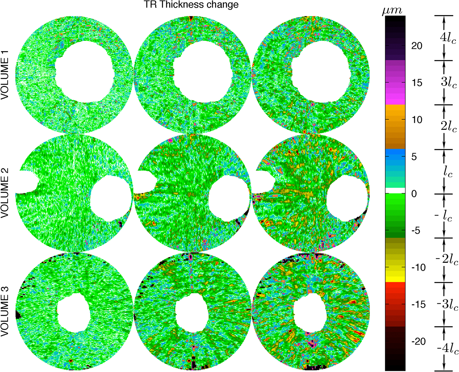$l_c=6\mu \text{m}$.

Table 2

Summary of the computed morphometric parameters: nerve fiber layer (NFL) thickness changes, total retinal (TR) thickness changes and cup to disc ratio for each of the three volumes, for different levels of subsampling.

	Scan area		Fully sampled	200 B-Scans	100 B-Scans	60 B-Scans
Volume 1	$4.4\times 4.4{\mathrm{mm}}^2$	Mean NFL thickness change (μm)	—	$0.8\pm 1.1$	$1.6\pm 2.0$	$2.3\pm 3.2$
		Mean TR thickness change (μm)	—	$1.8\pm 3.1$	$2.9\pm 4.3$	$4.0\pm 5.2$
		Cup to disc ratio $c/d$	0.18	0.17	0.17	0.17
Volume 2	$7.2\times 7.2{\mathrm{mm}}^2$	Mean NFL thickness change (μm)	—	$1.8\pm 3.5$	$4.0\pm 4.9$	$5.8\pm 6.9$
		Mean TR thickness change (μm)	—	$2.1\pm 3.8$	$4.5\pm 5.1$	$6.6\pm 7.1$
		Cup to disc ratio $c/d$	0.35	0.34	0.35	0.32
Volume 3	$7.2\times 7.2{\mathrm{mm}}^2$	Mean NFL thickness change (μm)	—	$2.3\pm 3.7$	$4.3\pm 5.5$	$5.9\pm 6.6$
		Mean TR thickness change (μm)	—	$3.2\pm 3.9$	$5.7\pm 5.6$	$7.9\pm 6.2$
		Cup to disc ratio $c/d$	0.21	0.20	0.20	0.20

The optic disc area was defined as the area of the region bounded by the BMO, and the optic cup area was defined as the area bounded by the ILM on the plane parallel and 150 μm anterior to the BMO plane.²⁹ The BMO plane was derived by performing principal component analysis on the BMO points. The cup-to-disc ratio ($c/d$) was calculated as the ratio of the optic cup area and optic disc area.²⁹ The $c/d$ values of the fully sampled and recovered volumes are also reported in Table 2.

To determine if the changes in $c/d$ values of the recovered volumes are significant, we compare our $c/d$ values to the $c/d$ values reported in Ref. 30. The authors of Ref. 30 performed a repeatability study to assess the intrasession variability of computing $c/d$. The authors reported a test-retest intrasession variability of 0.024 for healthy subjects. In our results, the greatest change in $c/d$ occurred in volume2 (0.35 for the fully sampled volume and 0.32 for the volume recovered from 60 radial B-scans). This change of $0.35-0.32=0.03$ in $c/d$ is slightly greater than the intrasession variability reported by Ref. 30, but is still of the same order. We thus come to the conclusion that, in terms of several clinically relevant measurements (TR thickness, NFL thickness and $c/d$ values), all the volumes were accurately reconstructed.

4.

Discussion

In this work, we have shown that using the theory of CS we can accurately reconstruct volumetric OCT images acquired from as few as 60 radial scans. Our method contains the main three ingredients required by the theory of CS: random sampling, sparsity of the signal in the representation basis, and the mutual incoherence between the sensing and sparsifying bases. In the proposed CS-based interpolation scheme, the OCT samples are acquired by randomly spaced radial B-scans, followed by a mapping into the ($r$, $\theta$, $z$) space where we perform the interpolation by minimizing the $l_1$-norm of the data’s wavelet coefficients subject to a data misfit, and then a mapping to the Cartesian coordinate system. We note that the use of $l_2$ norm in the data misfit term of Eq. (1) implies Gaussian nature of noise present in OCT. The main source of noise observed in OCT is speckle noise,³¹ and it has been previously demonstrated that speckle noise can be well modeled as additive white Gaussian noise with probability density function $N(0,{\sigma }^2)$^32,33 It has also been previously suggested that the true nature of noise present in photon-limited image acquisition systems (like OCT) in fact follows a Poisson distribution,³⁴ and subsequent promising sparsity-promoting image reconstruction methods from Poisson observations have been developed.^35,36 A detailed study on comparing reconstructed OCT images’ qualities from Gaussian and Poisson noise assumptions by sparsity-promoting inversion (CS) remain a topic of future research.

The acquisition geometry described in this work can be implemented with standard galvanometric mirrors used in commercial OCT systems, and does not require new hardware. Rapid radial acquisition/interpolation has several advantages over conventional raster-scanning methods. Prior to image acquisition the OCT system is aligned in such a way that the object of interest (in our case the optic nerve head) is located in the center of the image. Therefore when we acquire the volumetric OCT image each radial B-scan contains a depth profile for the object of interest. This greatly facilitates the morphometric analysis of the anatomical structures around the object of interest.¹⁵ Such a scan pattern results in dense sampling in the center of the image and fewer samples collected in the peripheral regions of the images. Due to the fact that there are relatively large gaps in data in the peripheral regions, if we were to perform the interpolation directly on the data acquired in Cartesian domain, the resulting interpolation quality would be poor in the regions further from the center. This is the primary motivation for mapping the radial scans to the ($r$, $\theta$, $z$) space and performing the interpolation there. This type of interpolation results in accurate reconstructions of B-scans not only in the center of the image but also in the peripheral regions, where the image sample spacing is high.

The reduction in scan time is directly proportional to the number of radial scans acquired when compared to the number of original raster scans. The percentage reduction in scan time can be calculated by the formula $(1-n/N)$ where $n$ is the number of acquired radial B-scans and $N$ is the number of original raster scans. For example, the original volume consisted of 382 raster scans, so the volume consisting of 60 radial scans corresponds to an $\sim 82\%$ reduction in scan time.

CS-based OCT image reconstruction from randomly spaced radial B-scans results in better image quality compared to regularly sampling a volume by radial B-scans, followed by linear interpolation. This can be seen from Fig. 11, which shows B-scans and C-scans extracted from the fully sampled volume, and from volumes that were acquired by 60 randomly spaced and 60 regularly spaced radial B-scans. The volume that was randomly sampled was interpolated with the $l_1$-minimization method described in this work, while the regularly sampled volume was interpolated by linear interpolation in the ($r$, $\theta$, $z$) space. Qualitatively, we observed that the CS-based image reconstruction technique was able to retain the anatomical structures of the image much more faithfully than the linear interpolation method, as can be seen in the structure of the ILMs shown in Fig. 11. Regular sampling, followed by linear interpolation resulted in image artifacts that degraded the smooth structure of the ILM, while random sampling with $l_1$-minimization recovery was able preserve the smoothness of the ILM much better. The primary reason for this is because linear, or any other local interpolation method relies on interpolating from image samples collected form directly adjacent B-scans, and with the methodology proposed in this paper this can only be done in one of the three dimensions, while the CS-based recovery is a 3-D global interpolation method, relying on image samples from all three dimensions and at different scales.

Fig. 11

(a) Fully acquired volume2. (b) 60 scans with CS-based interpolation. (c) 60 uniformly spaced scans with linear interpolation. The top row shows extracted C-scans while the bottom row shows extracted B-scans at the location of the yellow line. Notice how the linear interpolation degrades recovery whereas CS-based recovery presents a more faithful representation to the original data.

In terms of morphometric measurements such as TR thickness and NFL thickness, we found that most of the reconstructions’ computed parameters were below the intrinsic axial resolution ($l_c=6\mu \text{m}$) of the OCT system. The TR thickness of volume2 and volume3 reconstructed from 60 radial B-scans was slightly higher the intrinsic axial resolution of the OCT system, but still of the same order as $l_c$. We note that the errors in computed mean thicknesses are a convolution of errors from $l_1$-based image interpolation and the inaccuracies that arise in the segmentation algorithm.

5.

Conclusions

We have described a CS OCT scan pattern that consists of random-radial B-scans where the angle of a given B-scan, relative to the previous B-scan, is drawn randomly from a uniform distribution. This type of scan pattern is particularly suited for clinical studies where dense sampling in the center of a region is important. By acquiring and interpolating the data as described in Fig. 1, we are greatly facilitating the conversion of radial spokes to 3-D volumetric data for display and rendering purposes. Interpolation in Cartesian grid of the radial elements is a way of performing a cylindrical interpolation in the original radial space, and therefore, information of the underlying geometry, which is the optic nerve head, is propagated along cylindrical iso-distance lines leading to better interpolation. We have shown that recovering the data from a random-radial acquisition via CS-based interpolation achieves minimal degradation in the resulting image quality, which can subsequently lead to improved automatic segmentations^37–40 of relevant anatomical layers, and accurate computations of clinically relevant measurements of TR thickness, NFL thickness and $c/d$ values, which are often used as predictors for macular diseases such a glaucoma.²⁹ Furthermore, rapid volumetric image acquisition of the ONH is an important tool to investigate the role played by the morphology of the ONH in determining an individuals susceptibility to glaucoma.¹⁵ Reduction in the volumetric OCT scan time limits the discomfort of a subject during the scan and reduces the amount of motion artifacts. Due to the inherent radial geometry of the eye, this scan pattern is particularly suitable for imaging the optic nerve head. Although not demonstrated here, the technique is likely to have similar benefits for macular scanning. Extensions of this work could include investigating other representation bases that exploit the geometry of opthalmic OCT images. For example, due to the radial symmetry of the optic nerve head, discrete radial Bessel functions⁴¹ could be a natural choice to use as the representation basis of OCT images in the CS-based recovery. We speculate that the methods described in this paper could be beneficial for other imaging modalities like side-viewing OCT endoscopes,^42–44 intravascular ultrasound⁴⁵ and transrectal ultrasound,⁴⁶ where image samples are acquired in a radial fashion.