Algorithm for automated selection of application-specific fiber-optic reflectance probes

Andrew J. Gomes; Vadim Backman

doi:10.1117/1.JBO.18.2.027012

1 March 2013 Algorithm for automated selection of application-specific fiber-optic reflectance probes

Andrew J. Gomes, Vadim Backman

Author Affiliations +

Journal of Biomedical Optics, Vol. 18, Issue 2, 027012 (March 2013). https://doi.org/10.1117/1.JBO.18.2.027012

Abstract

Several optical techniques and fiber-optic probe systems have been designed to measure the optical properties of tissue. While a wide range of options is often beneficial, it poses a problem to investigators selecting which method to use for their biomedical application of interest. We present a methodology to optimally select a probe that matches the application requirements. Our method is based both on matching a probe’s mean sampling depth with the optimal diagnostic depth of the clinical application and on choosing a probe whose interrogation depth and path length is the least sensitive to alterations in the target medium’s optical properties. Satisfying these requirements ensures that the selected probe consistently assesses the relevant tissue volume with minimum variability. To aid in probe selection, we have developed a publicly available graphical user interface that takes the desired sampling depth and optical properties of the medium as its inputs and automatically ranks different techniques in their ability to robustly target the desired depth. Techniques investigated include single fiber spectroscopy, differential path length spectroscopy, polarization-gating, elastic light scattering spectroscopy, and diffuse reflectance. The software has been applied to biological case studies.

1. Introduction

A fiber-optic probe will interrogate a specific volume within a sample that is determined by the probe geometry and the sample optical properties. For accurate optical assessment of tissue structure and function, it is imperative that this interrogation volume coincides with the location where the relevant biological processes are occurring. The importance of depth-selectivity for accurate diagnosis has been underscored experimentally and clinically, especially for the early detection of cancer, which most often originates in a few-hundred-microns-thick mucosal tissue layer. Our optical and histological investigations in human patients and animal models of colon carcinogenesis have shown diagnostic alterations in hemoglobin concentration that are present in the mucosa but attenuated at deeper submucosal depths.¹^–⁵ Studies with angle-resolved low-coherence interferometry demonstrate that elevation of nuclear diameter associated with dysplasia in Barrett’s esophagus was only detectable at a depth of 200 to 300 μm and not observable at 0 to 100 μm or 100 to 200 μm.⁶ Several fiber-optic probe modalities have been developed to target the mucosal layer with a wide field of view. These include polarization-gating spectroscopy (PGS),⁷^,⁸ differential path length spectroscopy (DPS),⁹ elastic light scattering spectroscopy (ESS),¹⁰ single-fiber reflectance spectroscopy (SFS),¹¹ and angled-illumination-collection designs.¹²^–¹⁴ These methods have proven successful in diagnosing epithelial lesions including those in the colon, oral, and other types of mucosae.¹^,²^,⁹^,¹³^,¹⁵^–¹⁸ On the other hand, diffuse reflectance spectroscopy (DRS) methods typically have a sampling depth on the order of several millimeters and are consequently not very selective to the mucosal layer. However, the deeper sampling depth of DRS may be advantageous for other applications. For example, optical assessment of blood vessels under thick skin such as the palm requires light to first penetrate $\sim 1 mm$ through the epidermal layer. This can be achieved with DRS, but not easily with the other techniques mentioned previously. It is evident from the above considerations that matching the probe sampling depth to the clinical application is one of the main driving forces behind optimal probe selection.

Given the variety of spectroscopic methods that are currently available, there is a need to develop a schema for both choosing the correct technology and also selecting the optimal configuration of that technology for the application of interest. Parameters of the configuration can include size of the illumination-collection area, collection angle, fiber diameter, or inter-fiber spacing. In choosing an optical technology, there are a number of factors to consider including sampling depth, length-scale sensitivity, signal-to-noise ratio, cost, and convenience.

In the framework we develop in this paper, we focus on two crucial facets of probe development: the mean sampling depth and the sensitivity of the mean depth and path length to perturbations in the optical properties of the sample. Structurally and functionally, biological tissue is multilayered with specific biological processes and diseases occurring at different depth layers. Accurate optical assessment of these processes and diseases requires light to be preferentially targeted to the layer of interest making the sampling depth a critical aspect of probe design. It is important to point out that it is not sufficient to select a probe with an application-specific depth of tissue interrogation: one needs to consider how this sampling depth may vary depending on the optical properties of tissue. The clinical rationale for considering these parameters is that optimizing both of them will maximize the effect size for a given diagnostic parameter between control and disease groups. The Cohen effect size ( $d$ ) in statistics is defined as the difference in the means between the two groups divided by the pooled standard deviation ( $s$ ):

Eq. (1)

d = \frac{{\bar{x}}_{1} - {\bar{x}}_{2}}{s} .

Selecting an appropriate depth that targets the diagnostic layer will maximize

{\bar{x}}_{1} - {\bar{x}}_{2}

as highlighted by the clinical studies referenced previously. The effect size can also be improved by minimizing the pooled standard deviation. Previous research has focused on reducing biomarker variability through improved data collection,¹⁹^–²¹ calibration,²² and/or post-processing.²³ Another avenue to improve variability is by minimizing the dependence of the mean sampling depth and path length on the optical properties of the medium. This ensures that a consistent depth is targeted from tissue site to tissue site and also from patient to patient. In addition, robust application of the Beer-Lambert law to tissue spectroscopy requires that the path length be insensitive to tissue optical properties.²⁴ This fact has motivated the development of probe designs for which the path length is independent of optical properties.²⁵^,²⁶

It would be cumbersome to experimentally test side by side the individual technologies highlighted above for the optimum sampling depth and sampling depth sensitivity. To overcome this problem, we have culled the literature for mathematical expressions of the sampling depth and path length of various techniques and derived our own formulations. We have incorporated our analysis into a graphical user interface (GUI) that takes user input of the sample optical properties outputs optimum configurations of different spectroscopic techniques. The user can then select the best technique and configuration combination for their application of interest. We expect that our method and GUI tool will aid investigators who believe that optical methods would be useful in their disease screening research, but do not know which technique would be best suited for their task. Our results can also help researchers refine and optimize the geometry of their current fiber-optic probes.

2. Materials and Methods

2.1.

Probe Selection Metrics

A variety of factors can be considered when choosing a probe for a particular application. As stated in the introduction, we focused on the probe mean sampling depth and on the sensitivity of both the sampling depth and path length to perturbations in the optical properties of the medium. The main optical properties of a sample are the scattering coefficient $μ_{s}$ , the absorption coefficient $μ_{a}$ , and the average cosine of the scattering angle (anisotropy factor $g$ ). We found that the depth and path length were primarily functions of the reduced scattering coefficient $[μ_{s}^{'} = μ_{s} (1 - g)]$ and $μ_{a}$ . The problem of probe evaluation can be separated into two components, which need to be defined.

1. Mean sampling depth and path length calculation: We define the mean sampling depth as the expected value of the maximum depth reached by all collected photons in a Monte Carlo simulation:
Eq. (2)
$〈 Z 〉 = \frac{\sum_{i = 1}^{TPC} W_{i} Z_{i}}{\sum_{i = 1}^{TPC} W_{i}},$
with $W_{i}$ equal to the intensity weight of the $i$ th photon, $Z_{i}$ equal to the maximum depth reached by the $i$ ’th photon, and TPC being the total photons collected by the collection system. This definition of the mean depth has been used previously to characterize optical systems.⁷^,²⁷^–³² It has the advantage of being easy to visualize and can alert the user when the typical photon crosses a depth threshold. Other definitions, such as those based on the time spent at a depth $z$ or the depth at which specified percentage photons emerge from, are also possible.²⁵^,²⁸ Ideally, multiple definitions of the depth would be considered, requiring several models for each of the techniques presented. To maintain simplicity, we have used one of the accepted definitions of sampling depth and have applied it consistently across the different techniques studied. The definition of path length is the “mean average path length” pertinent to the modified Beer-Lambert Law for turbid media.³³^–³⁵ The modified Beer-Lambert Law has the form
Eq. (3)
$I = I_{s} \exp (- μ_{a} \bar{〈 L 〉}),$
where $I$ is the reflectance intensity, $I_{s}$ is the intensity that would be observed if the sample was devoid of absorbers, and $\bar{〈 L 〉}$ is the mean average path length defined as
Eq. (4)
$\bar{〈 L 〉} (μ_{a}, μ_{s}^{'}) = \frac{1}{μ_{a}} \int_{0}^{μ_{a}} 〈 L 〉 (μ_{a}^{'}, μ_{s}^{'}) d μ_{a}^{'},$
where $〈 L 〉 (μ_{a}, μ_{s}^{'})$ is the mean path length for a particular set of $(μ_{a}, μ_{s}^{'})$ .
2. Depth and path length sensitivity to optical properties calculation: We define the mean sampling depth and mean average path length sensitivity to a given sample optical property as the fractional change in the depth or path length given a small fractional change in the optical property of interest. As an example, the formula for the depth sensitivity to fluctuations in $μ_{a}$ for a sample having $μ_{a} = b_{1}$ and $μ_{s}^{'} = b_{2}$ is
Eq. (5)
$S_{μ_{a}}^{〈 Z 〉} = | \frac{\partial 〈 Z 〉 / {〈 Z 〉}_{μ_{a} = b_{1}, μ_{s}^{'} = b 2}}{\partial μ_{a} / b_{1}} |,$
where $b_{1}$ is the baseline magnitude of $μ_{a}$ , $b_{2}$ is the baseline level of $μ_{s}^{'}$ , and ${〈 Z 〉}_{μ_{a} = b_{1}, μ_{s}^{'} = b 2}$ is the depth evaluated at $μ_{a} = b_{1}$ and $μ_{s}^{'} = b_{2}$ . The sensitivity to $μ_{s}^{'}$ can also be calculated in the same fashion as Eq. (5), but with taking derivative of the depth with respect to $μ_{s}^{'}$ instead of $μ_{a}$ . The mean average path length sensitivity can also be determined by replacing $〈 Z 〉$ in Eq. (5) with $\bar{〈 L 〉}$ . The depth or path length will be independent of the optical properties of the sample if and only if the sensitivity as defined in Eq. (5) is equal to zero.

The probe selection criteria embodied by the mean sampling depth and the depth/path length sensitivities can automatically be calculated for a given optical technique if $〈 Z 〉$ and $\bar{〈 L 〉}$ are known. Expressions governing these parameters for DRS, PGS, ESS, SFS, and DPS are provided in the next section.

2.2.

Depth and Path Length Expressions

Expressions for the mean sampling depth and mean average path length of several optical spectroscopic techniques are given below. These expressions have been derived from MC simulations in which the sample was assumed to be homogeneous and in which the Henyey-Greenstein phase function was employed. In all cases, the illumination beam was assumed to have a flat intensity profile and the numerical aperture of simulated fibers was 0.22. The refractive index of the media was 1.4 to correspond to biological tissue, while the outside refractive index was 1.52 to correspond to either a lens or optical fiber.

1. DRS: DRS has been extensively used to extract optical properties from biological media. DRS probes have source-detector separations that are greater than $1 / μ_{s}^{'}$ to satisfy the assumptions of the diffusion approximation as shown in Fig. 1(a). Advantages of DRS include the ability to sample deeper tissue structures and the existence of well-characterized diffusion theory to help analyze reflectance data. The mean average path length for DRS in a semiinfinite geometry is³⁶^,³⁷
Eq. (6)
${\bar{〈 L 〉}}_{DRS} = 0.5 ρ {(\frac{3 μ_{s}^{'}}{μ_{a}})}^{0.5} [1 - \frac{1}{1 + ρ {(3 μ_{s}^{'} μ_{a})}^{0.5}}],$
where $ρ$ is the source-detector separation. The sampling depth for DRS has been given as³⁸
Eq. (7)
${〈 Z 〉}_{DRS} = \frac{1}{μ_{s}^{'}} {[\frac{π ρ μ_{s}^{'}}{2 μ_{eff} / μ_{s}^{'}}]}^{0.5},$
where $μ_{eff}$ is the effective attenuation coefficient equal to ${[3 μ_{a} (μ_{a} + μ_{s}^{'})]}^{0.5}$ .
2. Collimated illumination with overlapping illumination and collection areas: This is a broad category, and can include probes that use either polarized⁷ or unpolarized²⁵ light. In this configuration, a lens is typically used between the optical fibers and the sample surface to deliver a collimated illumination beam to the sample surface and to focus reflected light onto the collection fibers as shown in Fig. 1(b). The area on the sample surface that photons enter the sample and the area from which they emerge after being scattered overlap. Both the path length and the sampling depth of this method can be tuned by varying the radius (R) of the illumination-collection area and the collection angle ( $θ_{c}$ ). These in turn can be manipulated by the numerical aperture of the fibers, the lens focal length, and the spacing between illumination and collection fibers.³⁹ Path length and depth also depend on sample optical properties such as $μ_{s}^{'}$ , $μ_{a}$ , and the type of phase function. Our previous studies utilized a phase function based on the Whittle-Matérn model of light scattering from continuous refractive index media.⁴⁰ The shape of the refractive index correlation function, parameterized by the variable $m$ , influences the shape of the phase function. An $m$ value of 1.5 corresponds to the well-known Henyey-Greenstein (HG) phase function. Our group has previously developed equations for the mean average path length for the co-polarized reflectance signal ( $I_{∥}$ ), cross-polarized reflectance signal ( $I_{⊥}$ ), differential polarized-gated signal ( $Δ I = I_{∥} - I_{⊥}$ ), and the total reflectance signal ( $Σ I = I_{∥} + I_{⊥}$ ).⁴¹
Eq. (8)
${\bar{〈 L 〉}}_{Σ} = \frac{[2 (a_{2} \sqrt{R μ_{a}} - 1) {(R μ_{s}^{'})}^{a_{3}} \exp (a_{1} + a_{2} \sqrt{R μ_{a}})] - [- 2 {(R μ_{s}^{'})}^{a_{3}} \exp (a_{1})]}{a_{2}^{2} μ_{a}} .$
Eq. (9)
${\bar{〈 L 〉}}_{∥} = \frac{[2 (b_{2} \sqrt{R μ_{a}} - 1) {(R μ_{s}^{'})}^{b_{3}} \exp (b_{1} + b_{2} \sqrt{R μ_{a}})] - [- 2 {(R μ_{s}^{'})}^{b_{3}} \exp (b_{1})]}{b_{2}^{2} μ_{a}} .$
Eq. (10)
${\bar{〈 L 〉}}_{⊥} = \frac{(2 {c_{2} \sqrt{R μ_{a}} - [c_{1} + c_{3} \exp (- R μ_{s}^{'})] \ln [c_{1} + c_{2} \sqrt{R μ_{a}} + c_{3} \exp (- R μ_{s}^{'})]}) - (2 {- [c_{1} + c_{3} \exp (- R μ_{s}^{'})] \ln [c_{1} + c_{3} \exp (- R μ_{s}^{'})]})}{c_{2}^{2} μ_{a}} .$
Eq. (11)
${\bar{〈 L 〉}}_{Δ} = \frac{\ln (d_{1} + d_{2} R μ_{a} + d_{3} R μ_{s}^{'}) - \ln (d_{1} + d_{3} R μ_{s}^{'})}{d_{2} μ_{a}} .$
The parameters $[\begin{matrix} a_{n} & b_{n} & c_{n} & d_{n} \end{matrix}]$ are themselves functions of $θ_{c}$ and $m$ .⁴¹ For the purposes of our software algorithm, we fix $m$ to 1.5 (HG phase function) both because it has only a minor influence on the depth/path length (mean deviation of $< 12 %$ over the biological range of $m$ ) and to be able compare the polarization-gating results with other techniques that have mostly employed the HG phase function. In addition to the path length models, we have previously developed an expression for the differential polarization-gated signal which is the difference measurement between the co-polarized reflectance intensity and the cross-polarized reflectance intensity ( $Δ I = I_{‖} - I_{⊥}$ ). The mean sampling depth for the $Δ I$ signal was found to behave as a stretched exponential:³⁹
Eq. (12)
$τ^{'} = a {1 - \exp [- b {(R μ_{t}^{'})}^{c}]},$
where $μ_{t}^{'} = μ_{s}^{'} + μ_{a}$ , $τ^{'} = 〈 Z 〉 μ_{t}^{'}$ where $〈 Z 〉$ is the expected value of the maximum depth that photons will visit, and $[\begin{matrix} a & b & c \end{matrix}]$ are linear functions of $θ_{c}$ specified previously.³⁹ Following an general procedure as in Ref. 39, we have also developed expressions for the other polarization-gated signals:
Eq. (13)
$\frac{{〈 Z 〉}_{‖}}{R} = {(x_{1} + x_{2} R μ_{a} + x_{3} \sqrt{R μ_{s}^{'}})}^{- 1},$
Eq. (14)
$\frac{{〈 Z 〉}_{⊥}}{R} = {(y_{1} + y_{2} R μ_{a} + y_{3} \sqrt{R μ_{a}} + y_{4} \sqrt{R μ_{s}^{'}})}^{- 1},$
Eq. (15)
$\frac{{〈 Z 〉}_{\sum}}{R} = {(z_{1} + z_{2} R μ_{a} + z_{3} \sqrt{R μ_{s}^{'}})}^{- 1},$
where [ $x_{1}$ , $x_{2}$ , $x_{3}$ , $y_{1}$ , $y_{2}$ , $y_{3}$ , $z_{1}$ , $z_{2}$ , $z_{3}$ ] are functions of $θ_{c}$ . In brief, Eqs. (13) to (15) were derived from MC simulations that tracked the maximum depth collected photons travelled for many different combinations of $R μ_{s}^{'}$ and $R μ_{a}$ . A surface fitting procedure based on the least-squares technique was then used to find the functional forms that best fit the MC data. These functional forms are those given in Eqs. (13) to (15) and the coefficient values are listed in Table 1. Equations (8) and (15) can also be used in the case when unpolarized illumination and detection are used.⁴¹
3. SFS: This method uses a single fiber for both delivery and collection of light, as illustrated in Fig. 1(c). The advantage of SFS includes both the ability to have $< 1 - mm - diameter$ probes that can fit into endoscopic biopsy channels as well as catheters, and simple, cost-effective system design. The path length and sampling depth statistics of SFS have been studied with Monte Carlo simulations in which expressions for the mean average path length and mean sampling depth were formulated under the assumption of a HG phase function:³³
Eq. (16)
$\frac{{\bar{〈 L 〉}}_{SFS}}{d_{fiber}} = \frac{1.54}{{(μ_{s}^{'} d_{fiber})}^{0.18} [0.61 + {(μ_{a} d_{fiber})}^{0.61}]},$
Eq. (17)
${〈 z 〉}_{SFS} = \frac{0.38 \exp [- 0.06 (μ_{a} d_{fiber})]}{{(μ_{s}^{'} d_{fiber})}^{0.12}} {\bar{〈 L 〉}}_{SFS},$
where $d_{fiber}$ is the diameter of the fiber. Equation (17) was calculated on a different definition of the sampling depth based on a weighted mean. We found that this could be transformed to the expected value of the maximum depth by a multiplicative factor: ${〈 Z 〉}_{SFS} = {〈 z 〉}_{SFS} / 1.25$ on average.
4. DPS: A DPS probe consists of two adjacent fibers. One fiber serves as both a delivery and collection fiber (dc), while the remaining fiber only collects light (c) as depicted in Fig. 1(d). The tissue volume interrogated by the differential reflectance signal $dc - c$ has been found to be shallow and relatively independent of the optical properties of the medium.⁹ We simulated the DPS geometry with two fibers spaced $1.2 d_{fiber}$ apart owing to cladding separation.⁴² In contrast to Ref. 42, we also took into account the numerical aperture of the delivery and collection fiber ( $NA = 0.22$ ). In our MC modeling of the DPS geometry we found the DPS mean average path length to follow:
Eq. (18)
$\frac{{\bar{〈 L 〉}}_{DPS}}{d_{fiber}} = {[0.207 - 0.059 {(μ_{s}^{'} d_{fiber})}^{2} + 0.859 \sqrt{μ_{s}^{'} d_{fiber}} + 0.317 μ_{a} d_{fiber}]}^{- 1} .$
An empirical equation for the DPS path length has also been provided for a fixed $g = 0.8$ :⁴³
Eq. (19)
$\frac{{\bar{〈 L 〉}}_{DPS}}{d_{fiber}} (g = 0.8) = \frac{1 + {(μ_{s} d_{fiber})}^{- 0.53}}{1 + {(μ_{a} d_{fiber})}^{0.53}} .$
The drawback of the empirical equation is that it is only valid for $g = 0.8$ , whereas the model in Eq. (18) has the $g$ variable incorporated in $μ_{s}^{'}$ . We have observed that the path length can increase by greater than 20% when $g$ is increased from 0.8 to greater than 0.9. Many tissues have $g$ in the range of 0.9. Therefore, we have decided to use Eq. (18) instead of Eq. (19) in our algorithm since it is valid across a wider range of $g$ values encountered in biological tissue. When the $g$ value is fixed to 0.8 in Eq. (18), we obtain excellent agreement with the experimental results of Eq. (19) with a mean percent error of 8% and a maximum percent error of only 17% across the entire range of $μ_{s} d_{fiber}$ and $μ_{a} d_{fiber}$ studied in Ref. 43. This agreement experimentally validates Eq. (18) for $g = 0.8$ and underscores the validity of our MC modeling of the DPS probe geometry. Simulations revealed the DPS sampling depth to be of the following form:
Eq. (20)
$\frac{{〈 Z 〉}_{DPS}}{d_{fiber}} = {(0.337 + 1.95 \sqrt{μ_{s}^{'} d_{fiber}} + 1.56 μ_{a} d_{fiber})}^{- 1} .$
Equations (18) and (20) were derived from simulations having $d_{fiber} = [0.01, 0.04, 0.06, 0.08, 0.1] cm$ , $g = [0.8, 0.9, 0.95]$ , $μ_{s} = [50, 100, 250] {cm}^{- 1}$ , and $μ_{a} = [0 - 40] {cm}^{- 1}$ .
5. ESS: Probes based on ESS typically have small source and detector fiber separation ( $ρ < 1 / μ_{s}^{'}$ ), which allows them to sample superficial tissue layers. The basic geometry of an ESS probe is shown in Fig. 1(e). In theory, the depth and path length can be turned by the fiber diameter, center-to-center fiber spacing, and fiber tilt.¹⁰ In our Monte Carlo analysis we restricted the fiber diameter to 200 μm and the fiber tilt to 0 deg, as these are the most typically used configurations. We then charted the sampling depth and path length as a function of the center-to-center fiber separation $ρ$ . We found that we could leverage Eqs. (16) and (17) from SFS ( $ρ = 0$ ) such that
Eq. (21)
$\begin{array}{l} {\bar{〈 L 〉}}_{ESS} = {\bar{〈 L 〉}}_{SFS} (0.0051 ρ + 1.88) \\ {〈 Z 〉}_{ESS} = {〈 Z 〉}_{SFS} (0.0021 ρ + 2.12), \end{array}$
where $ρ$ is in units of microns. Equation (21) was derived from MC simulations of the ESS geometry with $ρ = [250, 500, 750, 1000, 1250, 1500] μ m$ on media having $g = [0.8, 0.9, 0.95]$ , $μ_{a} = 1 - 20 {cm}^{- 1}$ and $μ_{s} = [50, 100, 200] {cm}^{- 1}$ .

Fig. 1

Probe geometries of the different optical techniques investigated. (a) Diffuse reflectance spectroscopy (DRS). (b) Polarization-gating spectroscopy (PGS). (c) Single-fiber reflectance spectroscopy (SFS). (d) Differential path length spectroscopy (DPS). (e) Elastic light scattering spectroscopy (ESS).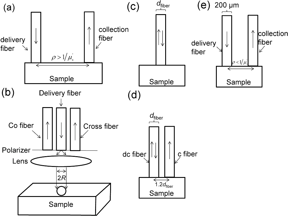

Table 1

Fitting coefficients for PGS depth models.

Parameter	Functional form
$x_{1}$	${[- 13.9 + 62.9 / \ln (θ_{c})]}^{- 1}$
$x_{2}$	$2.30 + 0.00075 θ_{c}^{2}$
$x_{3}$	${(0.71 + 0.028 \sqrt{θ_{c}})}^{- 1}$
$y_{1}$	${(- 10.06 + 0.38 \sqrt{θ_{c}})}^{- 1}$
$y_{2}$	${(0.93 - 0.0066 θ_{c})}^{- 1}$
$y_{3}$	$0.61 + 5.65 \cdot 10^{- 6} θ_{c}^{3}$
$y_{4}$	${(1.16 - 8.58 \cdot 10^{- 5} θ_{c}^{2})}^{- 1}$
$z_{1}$	$\exp (- 3.45 + 0.36 \sqrt{θ_{c}})$
$z_{2}$	$2.45 + 0.00075 θ_{c}^{2}$
$z_{3}$	1

2.3.

Probe Selection Algorithm

Selecting an optimal probe is a multicriteria decision analysis problem. One method to solve such problems is a weighted sum model (WSM). In the WSM, each criterion is given a relative weight of importance. There are two main criteria in our probe selection problem.

1. Deviation of the mean sampling depth from the target depth: A given probe will have an mean sampling depth characterized by $〈 Z 〉$ . The user of that probe will have a target depth ( $P_{t}$ ) within the sample that they are trying to interrogate. The deviation of the probe depth from the target depth can be calculated as $(| P_{t} - 〈 Z 〉 |) / P_{t}$ . For an ideal probe, the deviation would be zero.
2. Sensitivities of the sampling depth and path length to $μ_{s}^{'}$ and $μ_{a}$ : The sensitivities can be calculated according to Eq. (5). The properties $μ_{s}^{'}$ and $μ_{a}$ are chosen because the sampling depth and path length equations can be reduced to functions of these two parameters. An ideal probe would have all calculated sensitivities equal to zero such that the depth and path length are independent of the sample optical properties.

The sampling depth deviation as well as depth and path length sensitivities will be functions of the probe geometry $G$ for each optical technique. The geometry can be manipulated by changing $R$ , $d_{fiber}$ , $θ_{c}$ , or $ρ$ . Suppose that a user has a target depth of $P_{t}$ and that probe geometry $G$ has sampling depth $〈 Z 〉 (G)$ , depth sensitivities $S_{μ_{s}^{'}}^{〈 z 〉} (G)$ and $S_{μ_{a}}^{〈 z 〉} (G)$ , and path length sensitivities $S_{μ_{s}^{'}}^{\bar{〈 L 〉}} (G)$ and $S_{μ_{a}}^{\bar{〈 L 〉}} (G)$ . In our analysis, optimal probe selection will be achieved by choosing a particular $G$ to minimize the weighted sum $A (G)$ :

Eq. (22)

A (G) = w_{1} \frac{| P_{t} - 〈 Z 〉 (G) |}{P_{t}} + w_{2} S_{μ_{s}^{'}}^{〈 z 〉} (G) + w_{3} S_{μ_{a}}^{〈 z 〉} (G) + w_{4} S_{μ_{s}^{'}}^{\bar{〈 L 〉}} (G) + w_{5} S_{μ_{a}}^{\bar{〈 L 〉}} (G),

where

w_{1} - w_{5}

are relative weights supplied by the user. These weights indicate the importance the user places on the corresponding criteria term. For example, if

w_{1}

is set to zero, then the algorithm will not take into consideration the match between the target depth and the probe sampling depth when selecting an optimal geometry. In contrast, if

w_{1}

is set to a high value, the algorithm will attempt to match the target depth and the probe sampling depth very accurately. To minimize Eq. (22), we used the Nelder-Mead optimization algorithm in MATLAB. In brief, the algorithm will cycle (via a simplex search) through the geometry parameters (

d_{fiber}

,

ρ

,

R

, and

θ_{c}

) until a minimum sum is reached. It will do this separately for each optical technique such that there will be an optimum geometry for DRS, PGS, SFS, DPS, and ESS.

2.4.

Automated Probe Selection with a MATLAB Graphical User Interface

We implemented a MATLAB GUI to automate probe selection using Eq. (22). A screenshot of the GUI is shown in Fig. 2(a). The first step in the GUI is for the user to specify the baseline values of, and $μ_{a}$ which in turn delineate the $b_{1}$ and $b_{2}$ parameters of Eq. (5). These values should correspond with mean optical properties of the sample of interest and can be obtained from the literature or experimentally determined integrating sphere measurements. The optical properties of a wide variety of tissue types have been previously studied.⁴⁴ However, care must be taken when translating ex vivo optical property determinations to in vivo measurements. The second step is for the use to enter the target depth. The target depth is the depth within the sample where the most diagnostic or scientifically relevant information is expected to be obtained. Next, the user stipulates the relative weights given in Eq. (22). These weights determine the criteria that will be the most important in the automated selection process. If these are not explicitly specified, they will default to a value of 1. Finally, the user can place upper and lower bounds on the probe geometry parameters such as $d_{fiber}$ , $ρ$ , $R$ , and $θ_{c}$ . This may help the user limit the selection space to geometries that utilize commercially available components or that are more convenient in a clinical setting. After all input values have been selected and the user initiates the automated selection, the program will attempt to minimize Eq. (22) for each optical technique. After the minimization procedure is complete, the GUI will output a table of results as depicted in Fig. 2(a). Each row of the table corresponds to a different optical technique (DRS, PGS, SFS, DPS, ESS). The first column gives the weighted sum from Eq. (22) for the optimal geometry of each technique. The best technique will have the lowest value in the first column. The next five columns give the values of the optimization criteria: the depth deviation and the depth and path length sensitivities. In the remaining columns are shown the values of the geometry parameters ( $d_{fiber}$ , $ρ$ , $R$ , and $θ_{c}$ ) that compose the optimum geometry. The user can take these values and construct the ideal application-specific probe.

Fig. 2

MATLAB graphical user interface (GUI) for automated probe selection. (a) GUI interface where the user can enter the target depth, optical properties for the medium, weights for the optimization algorithm, and bounds on the probe geometry parameters. Pressing the submit button will initiate the algorithm and the results will be outputted to the depicted table. (b) The “depth and path length spectra” panel in the GUI allows the user to plot the depth or path length spectrum for a selected technique by loading a data file consisting of the optical properties as a function of wavelength. Depicted is the SFS path length spectrum.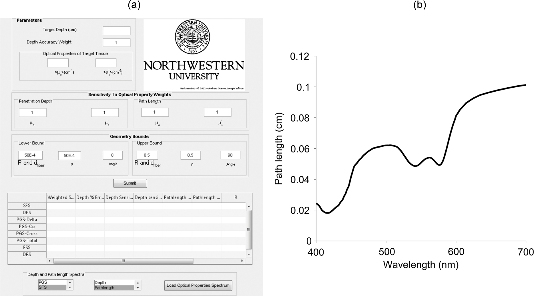

The DRS technique is known to be valid across a specified range of parameters. Therefore, in our algorithm we institute two checks to make sure the user is notified as to when the diffuse reflectance assumptions may be violated. The algorithm displays a warning dialog box if the transport albedo $(μ_{s}^{'} / μ_{s}^{'} + μ_{a}) < 0.8$ for which the DRS result would not be accurate.⁴⁵ In addition, the algorithm ensures that the output value of $ρ$ satisfies $ρ μ_{s}^{'} > 1$ . A warning dialog is displayed if the upper and lower bounds on $ρ$ would not satisfy this property.

The algorithm outputs ideal probe configurations based on single values for $μ_{s}^{'}$ and $μ_{a}$ that correspond to a single wavelength. Since broadband measurements are often taken, it can be useful to visualize how the depth and path length vary with wavelength. To satisfy this need, the GUI plots the depth and/or path length for each technique as a function of wavelength. This is achieved in the “depth and path length spectra” panel of the GUI, as shown in Fig. 2(a). The user selects a technique from the first drop-down menu, either the depth or path length from the second drop-down menu, and then loads a MATLAB data file. The data file consists of the wavelength in the first column followed by the corresponding $μ_{s}^{'}$ and $μ_{a}$ values in the second and third columns, respectively. Based on these values, the GUI will use the expressions in Sec. 2.1 to calculate the depth or path length at each wavelength for the ideal geometry specified in the GUI table. As an example, we show the SFS path length spectra for $d_{fiber} = 400 μ m$ in Fig. 2(b). The value of $μ_{s}^{'}$ was $20 {cm}^{- 1}$ at 560 nm and followed a $λ^{- 1}$ dependence. The value $μ_{a}$ was $10 {cm}^{- 1}$ at 560 nm and followed the absorption spectrum of hemoglobin with 75% oxygen saturation. The path length follows the hemoglobin spectrum with dips in the path length corresponding to the characteristic hemoglobin absorption peaks at 420, 542, and 576 nm.

2.5.

Case Studies

To illustrate the use of the GUI, we consider two biological case studies. The first is the case of detecting dyplasia in Barrett’s esophagus. Previous research with angle-resolved low coherence interferometry has shown that diagnostic increases in nuclear size occur at a depth of 200 to 300 μm beneath the esophageal surface.⁶ The user could set a target depth of 250 μm in the GUI. The optical properties at a wavelength of 630 nm for normal human esophagus have been supplied by Table 2 of Holmer et al.: $μ_{a} = {2.1 \pm 3.6 cm}^{- 1}$ , $μ_{s} = {125.6 \pm 22.3 cm}^{- 1}$ , and $g = 0.94 \pm 0.02$ .⁴⁶ The next task is assigning the relative weights from Eq. (22). It has been found that the diagnostic changes occurring with esophageal dysplasia are localized to the 200- to 300-μm layer. Therefore, it is important to have the target depth and probe sampling depth match as closely as possible and we set $w_{1} = 1$ . Assigning weights to the sensitivity variables hinges on several considerations. The standard of deviation $μ_{a}$ is high with a coefficient of variation greater than one. To maintain a consistent depth or path length given this variability, it is desirable minimize the sensitivity of the depth and path length to $μ_{a}$ . The increase in nuclear size observed with low coherence interferometry might be expected to result in an increase in $g$ and consequent reduction in $μ_{s}^{'}$ . To target the same region between control and dysplastic patients would necessitate minimizing the depth and path length sensitivity to $μ_{s}^{'}$ . For simplicity, we will set $w_{2} - w_{5}$ also equal to one. The final user input is setting bounds on the geometry parameters. Choice of these bounds is primarily driven by what is commercially available or feasible to manufacture and what is clinically convenient. For example, the diameter of upper endoscope accessory channels places upper bounds on the size of a potential esophageal probe. We set a lower limit of 100 μm and upper limit of 3 mm for $d_{fiber}$ and $R$ while setting the lower limit of $ρ$ to 250 μm. We allowed $θ_{c}$ to vary from 0 deg to 45 deg.

Table 2

Algorithm results for esophageal dysplasia detection case study.

			Depth sensitivity		Path length sensitivity
Technique	Weighted sum	Depth % error	$μ_{s}^{'}$	$μ_{a}$	$μ_{s}^{'}$	$μ_{a}$	$R$ (cm)	$d_{fiber}$ (cm)	$p$ (cm)	$θ_{c}$
SFS	0.746	7.090E-3	0.300	0.134	0.180	0.131	NA	0.025	NA	NA
DPS	0.785	3.830E-3	0.346	0.082	0.320	0.036	NA	0.037	NA	NA
PGS-Delta	0.921	2.513E-8	0.420	0.117	0.328	0.055	0.017	NA	NA	11.366
PGS-Co	0.715	3.104E-8	0.224	0.206	0.156	0.129	0.029	NA	NA	46.334
PGS-Cross	1.277	1.240E-5	0.301	0.346	0.299	0.331	0.018	NA	NA	60.000
PGS-Total	0.702	4.477E-7	0.253	0.171	0.167	0.110	0.018	NA	NA	32.864
ESS	2.020	130.7	0.300	0.119	0.180	0.117	NA	NA	0.025	NA
DRS	3.205	184.0	0.253	0.111	0.927	0.073	NA	NA	0.025	NA

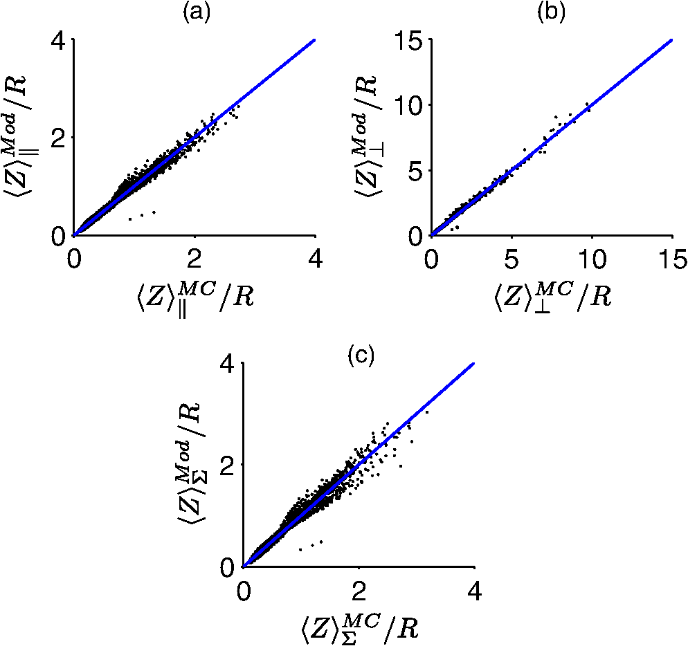
The second case involves optically determining chromophore concentrations from target tissue using a Beer’s Law algorithm. This approach has been previously used to study microcirculatory alterations associated with dysplasia²^,⁴⁷ as well as to monitor chemotherapy drug concentrations in tissue.⁴⁸ Insensitivity of the effective path length to tissue optical properties helps to ensure robust application of this method.²⁴^,²⁶ For the second case study, we change the target depth to 150 μm. Hemoglobin concentration measured from this depth was diagnostic for early detection of colonic neoplasia.² For simplicity, we will maintain the same optical properties as the first case study since the optical properties of the colon have been found to be similar.⁴⁹ In general, the optical properties will need to be adjusted based on the tissue or organ being investigated. This case study will require higher weights to be placed on the path length sensitivity terms. As an example, we will consider $w_{1} = 0.5$ , $w_{2} = w_{3} = 0.1$ and $w_{4} = w_{5} = 1$ .

3. Results

3.1.

Validation of Sampling Depth Expressions for PGS

In Fig. 3, we plot the MC simulations of the PGS sampling depth versus the models developed in Eqs. (13) to (15). Each PGS signal is shown in a different subplot of Fig. 3. with (a) co-polarized signal, (b) the cross-polarized signal, (c) total signal. In all cases, there is a clear linear correlation between the simulations and the models with Pearson correlation coefficient greater than 0.99. The mean percent differences between model and simulation were 9% for the co-polarized signal, 8% for the cross-polarized signal, 10% for the total signal. The error for the delta-polarized signal has been previously found to be ~5% in Ref. 39. This leads us to conclude that Eqs. (13) to (15) can be used as accurate condensations of the MC simulations for PGS.

Fig. 3

Comparison of sampling depth model estimates ( ${〈 Z 〉}^{Mod}$ ) for polarization-gated measurements shown in Eqs. (13) to (15) with the Monte Carlo simulation estimates ( ${〈 Z 〉}^{MC}$ ): (a) co-polarized signal, (b) cross-polarized signal, (c) total polarized signal. The line of unity is shown for comparative purposes.

3.2.

Validation of Depth and Path Length Expressions for DPS

We illustrate the correspondence between our MC simulations of the DPS geometry and the models of Eqs. (18) to (20) for the depth and path length in Fig. 4(a) and 4(b). Figure 4(a) demonstrates that the simulation and model coordinates cluster around the ideal line of unity indicating good agreement. This agreement was quantified through the mean percent error, which was 3%. Figure 4(b) also demonstrates good agreement between simulation and model with an overall percent error of 3% for the path length. As previously mentioned in Sec. 2.2, our model of the DPS path length agrees well with previously published experimental data⁴³ with a mean percent error of 8%.

Fig. 4

Comparison of the models developed in Eqs. (18) to (20) for the differential path length spectroscopy (DPS) mean sampling depth and mean average path length with the Monte Carlo results from simulations of the DPS probe geometry. (a) Monte Carlo simulations of DPS depth ( ${〈 Z 〉}_{DPS}^{MC} / d_{fiber}$ ) versus model predictions of the DPS depth ( ${〈 Z 〉}_{DPS}^{Mod} / d_{fiber}$ ). (b) Monte Carlo simulations of the DPS mean average path length ( ${\bar{〈 L 〉}}_{DPS}^{MC} / d_{fiber}$ ) versus model predictions of the DPS mean average path length ( ${\bar{〈 L 〉}}_{DPS}^{Mod} / d_{fiber}$ ). The line of unity is shown for comparative purposes.

3.3.

Validation of Depth and Path Length Expressions for ESS

In Fig. 5(a) and 5(b) we have plotted our MC simulations of the depth and path length of the ESS geometry versus our models of the depth and path length from Eq. (21). For the depth plotted in Fig. 5(a), there is a 9% error percent difference of the depth data points about the ideal line of unity. In Fig. 5(b), the percent difference of the path length data about the unity line is 11%. Figure 5(b) also plots the path length as determined from a previously published analytical model for ESS by Reif et al.:¹⁰ $\bar{〈 L 〉} = [0.32 / {(μ_{a} μ_{s}^{'})}^{0.21}]$ . This equation is only valid for 200-μm diameter fiber with a 250-μm inter-fiber spacing. As Fig. 5(b) demonstrates, the data points from this previously validated model (shown in red) clearly overlap with the data points from model in Eq. (21) (shown in black). This underscores the validity of our MC simulations of the ESS geometry and the models we derived from them.

Fig. 5

Comparison of the models developed in Eq. (21) for the elastic scattering spectroscopy (ESS) mean sampling depth and mean average path length with the Monte Carlo results from simulations of the ESS probe geometry. (a) Monte Carlo simulations of ESS depth ( ${〈 Z 〉}_{ESS}^{MC} / d_{fiber}$ ) versus model predictions of the ESS depth ( ${〈 Z 〉}_{ESS}^{Mod} / d_{fiber}$ ). (b) In black are the Monte Carlo simulations of the ESS mean average path length ( ${\bar{〈 L 〉}}_{ESS}^{MC} / d_{fiber}$ ) versus model predictions [Eq. (21)] of the ESS mean average path length ( ${\bar{〈 L 〉}}_{ESS}^{Mod} / d_{fiber}$ ). In red are the Monte Carlo simulated path length versus the path length predicted by Ref. 10 for an ESS probe with $d_{fiber} = 200 μ m$ and inter-fiber spacing of 250 μm. The line of unity is shown for comparative purposes.

3.4.

Sampling Depth and Sensitivity Behavior

We now examine the behavior of the mean sampling depth for all the techniques previously mentioned. In particular, we were interested in how the depth could be tuned by varying the geometry, as this would directly affect optimal probe selection. In Fig. 6, we plot the log of the sampling depth scaled by $μ_{s}^{'}$ of the various techniques versus a parameter we term the area extent. The area extent is a measure of the maximum horizontal distance a photon could travel between its entry and exit points for each technique multiplied by $μ_{s}^{'}$ . For PGS the area extent is equal to $2 R μ_{s}^{'}$ , for DPS and SFS the area extent is $μ_{s}^{'}$ $d_{fiber}$ , while for ESS and DRS the area extent is $ρ μ_{s}^{'}$ . From the expressions in Sec. 2.1 it can be observed that in the case of PGS, SFS, and DPS, for $μ_{a} \to 0$ , the quantity $μ_{s}^{'} 〈 Z 〉$ can be represented as a function solely of the area extent. The optical properties used to generate the data in Fig. 6 are $μ_{s} = 200 {cm}^{- 1}$ , $μ_{a} = 0$ , and $g = 0.9$ From Fig. 6, it is clear that the sampling depth increases with the area extent for all the techniques though the precise behavior is not the same. For example, the delta-polarized signal saturates very quickly with area extent when compared with other methods.

Fig. 6

Area extent versus mean sampling depth for each technique included in the probe selection algorithm. The definition of area extent is defined as the size of the illumination-collection area ( $2 R$ , $d_{fiber}$ , or $ρ$ ) multiplied by $μ_{s}^{'}$ .

Next we wanted to examine the sensitivity of the depth and path length to $μ_{s}^{'}$ and $μ_{a}$ . In Fig. 7(a) and 7(b) we plot the sensitivity [defined in Eq. (5)] of the sampling depth to $μ_{s}^{'}$ and $μ_{a}$ , respectively, as a function of a geometry parameter. The geometry parameter is simply defined as $2 R$ for PGS, $d_{fiber}$ for DPS and SFS, and $ρ$ for DRS. The ESS technique is not shown since its sensitivity will be identical to that of SFS over the range of $ρ$ specified in Sec. 2.2. The optical properties used to generate the data in Fig. 7 are $μ_{s} = 200 {cm}^{- 1}$ , $μ_{a} = 2 {cm}^{- 1}$ , and $g = 0.9$ . Examination of Fig. 7(a) shows the dependence of the $μ_{s}^{'}$ depth sensitivity on the geometry parameter is dependent on the technique being used. In most cases, the sensitivity decreases when the geometry parameter is increased. Notable exceptions are the PGS delta-polarized signal for which the sensitivity increases and eventually saturates with $R$ and SFS/ESS and DRS for which the sensitivity is independent of $d_{fiber}$ . If the main objective was to minimize $μ_{s}^{'}$ depth sensitivity, then selection of a DRS probe or analysis of the total-polarization signal from a polarization-gated probe with area extent greater than five would be appropriate. It should be noted that the validity of the DRS equations used to generate Figs. 6 and 7 are applicable when the diffusion approximation is valid, namely when $ρ μ_{s}^{'} ≫ 1$ . Next we examine the $μ_{a}$ depth sensitivity depicted in Fig. 7(b). Here the behavior of the sensitivity as a function of the geometry parameter is more uniform across optical techniques. In nearly all cases, the sensitivity increases with the geometry parameters. The lone exception is DRS, for which the depth sensitivity is independent of $ρ$ . Optimal minimization of the $μ_{a}$ depth sensitivity would entail selection of a DRS probe.

Fig. 7

Sensitivities of the mean sampling depth and mean average path length for each optical technique to perturbations in $μ_{s}^{'}$ and $μ_{a}$ plotted as functions of the geometry parameter. The geometry parameter is defined as $R$ , $d_{fiber}$ , or $ρ$ depending on the technique. (a) Depth sensitivity to $μ_{s}^{'}$ . (b) Depth sensitivity to $μ_{a}$ . (c) Path length sensitivity to $μ_{s}^{'}$ . (d) Path length sensitivity to 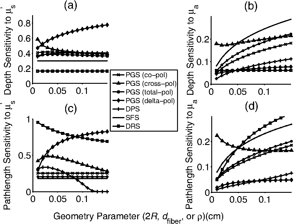$μ_{a}$ .

Next, we explored the sensitivity of the path length to $μ_{s}^{'}$ and $μ_{a}$ in Fig. 7(c) and 7(d), respectively. The SFS/ESS, PGS (co-pol), and PGS (total-pol) methods have path length $μ_{s}^{'}$ sensitivities that are independent of the geometry parameter. The PGS (delta-pol) sensitivity increases with $R$ and saturates at large $R$ . The DRS sensitivity steadily decreases with $ρ$ , while the PGS (cross-pol) and DPS tend to decrease with the geometry parameter. The behavior of the DPS path length sensitivity to $μ_{s}^{'}$ deserves further examination. The DPS sensitivity reaches zero when $μ_{s}^{'} d_{fiber}$ is approximately equal to 2.4 or equivalently when the transport mean free path [ $l^{*} = (1 / μ_{s}^{'})$ ] is equal to $2.4 d_{fiber}$ , which corresponds to twice the center-to-center separation between the DPS fibers. It is beyond the scope of this paper to confirm whether this phenomenon generalizes to other inter-fiber spacings, but it is useful to know where exactly the sensitivity reaches the optimal zero value. Finally, we investigated $μ_{a}$ path length sensitivity in Fig. 7(d). The main pattern observed is for the sensitivity to increase with the geometry parameter for all the optical methods. The optimal techniques for $μ_{a}$ path length sensitivity minimization are DPS and the PGS (delta-pol) methods.

3.5.

Application of Automated Probe Selection Algorithm to Biological Case Studies

We utilized the MATLAB GUI to implement the probe selection algorithm embodied in Eq. (22). For the case of detecting dysplasia in Barrett’s esophagus, we input the optical properties, target depth, and associated weights as described in Sec. 2.5. The automated algorithm took 0.15 s to run on a personal computer and the results were outputted in tabular format. These results are summarized in Table 2. Each row corresponds to a different technique, and each column gives the value of the criterion or geometry parameter for the optimal geometry of that technique. The optimal technique will have the lowest value in the weighted sum column. For this case study, the PGS-total, PGS-co, and SFS techniques performed similarly with weighted sum equal to ~0.7. The ideal SFS probe would have a $d_{fiber}$ of 0.025 cm. In general, most of the optical methods are capable of targeting the specified depth with an error less than 1%. The exceptions are ESS and DRS. This is because they tend to target deeper depths than the specified 0.025 cm. The next case study we examined was measuring chromophores concentration from a shallow depth of 0.0150 cm. Compared to the first case, the target depth was less and higher weight was placed on the path length sensitivity. The results of this case study are depicted in Table 3. For this case study, a PGS (delta-pol) probe with an $R$ of 0.005 cm and $θ_{c} = 6 \deg$ is optimal. Using this type of probe, the 0.0150-cm depth would be interrogated within 1%. For a 1% perturbation in $μ_{s}^{'}$ or $μ_{a}$ , the path length of the PGS (delta-pol) probe would deviate by 0.15% and 0.02%, respectively.

Table 3

Algorithm results for chromophores concentration measurement at a depth of 150 μm.

			Depth sensitivity		Path length sensitivity
Technique	Weighted sum	Depth % error	$μ_{s}^{'}$	$μ_{a}$	$μ_{s}^{'}$	$μ_{a}$	$R$ (cm)	$d_{fiber}$ (cm)	$p$ (cm)	$θ_{c}$
SFS	0.304	0.017	0.300	0.086	0.180	0.085	NA	0.011	NA	NA
DPS	0.317	0.012	0.317	0.049	0.260	0.021	NA	0.016	NA	NA
PGS-Delta	0.224	1.988E-7	0.377	0.105	0.151	0.024	0.005	NA	NA	5.8
PGS-Co	0.272	1.115E-6	0.175	0.144	0.139	0.101	0.017	NA	NA	54.9
PGS-Cross	0.725	13.0	0.387	0.384	0.212	0.371	0.005	NA	NA	60.0
PGS-Total	0.272	1.377E-6	0.203	0.123	0.154	0.085	0.010	NA	NA	44.0
ESS	1.760	284.4	0.300	0.119	0.180	0.117	NA	NA	0.025	NA
DRS	2.903	373.0	0.253	0.111	0.927	0.073	NA	NA	0.025	NA

4. Discussion

In this paper, we have provided a simple and flexible framework for application-specific fiber-optic probe design. The guiding principle of the algorithm was to maximize diagnostic effect size for clinical biophotonic applications as defined in Eq. (1). To accomplish this, our framework takes into account the target sampling depth, and the sensitivity of the depth and path length to fluctuations in the optical properties of the sample. We use a weighted sum algorithm incorporating the above criteria to optimize the probe geometry. The algorithm is implemented in an easy-to-use MATLAB GUI interface where the user can specify the target depth, sample optical properties, relative importance of the algorithm criteria, and bounds on elements of the probe geometry. We plan on making this software publicly available for researchers to use.

Our results show that in most cast cases, both the mean sampling depth and the sensitivities of the path length and depth can be adjusted by the geometry. Notable exceptions include PGS (co-pol), PGS (total-pol), and SFS for which the path length sensitivity is independent of this value. In general, depth and path length sensitivity to $μ_{a}$ increases with the geometry parameter ( $2 R$ , $d_{fiber}$ , or $ρ$ ) for all optical techniques. The pattern is more complicated when looking at the sensitivity to $μ_{s}^{'}$ . Here the sensitivity may decrease or increase with the geometry parameter depending on the optical technique. For example, the path length sensitivity increases with $R$ for the PGS (delta-pol) signal but decreases with $d_{fiber}$ for the DPS method. In addition, a wide range of depths. ESS and DRS tend to sample depths greater than $l^{*}$ , while the remaining methods interrogate depths on the order of 0.3-1 $l^{*}$ as shown in Fig. 6.

The biological case studies we laid out gave realistic and concrete examples of probe selection scenarios. The first example was diagnosing esophageal dysplasia at a depth of 250 μm. All the techniques except for ESS and DRS had a depth percent error of less than 3%. This is not surprising, as these methods were designed largely in part to target mucosal tissue structures. If we had set a deeper target depth, then the ESS and DRS techniques would have performed better. Indeed, if the target depth is set to 650 μm, the depth percent error for ESS drops from 131% to 5%. Our next case study involved measuring chromophore concentration from a depth of 150 μm. In this example, the path length sensitivity was considered paramount for accurate application of Beer’s law. The PGS (delta-pol) was found to be ideal both because of its ability to correctly achieve the 150-μm depth and its low path length sensitivity to $μ_{a}$ . At this juncture, it must be stressed that the outcome of the algorithm depends on the user-selected weights of Eq. (22). This is both an advantage and disadvantage. The advantage is that it gives the user a lot of flexibility to experiment with different weights and find what best matches the application. This, however, introduces an element of subjectivity to the problem of probe selection in the quality of the output depends on user guidance. In addition, the algorithm will be sensitive to the accuracy of the tissue optical properties input by the user. In general, the optical properties are not known precisely and must be estimated, typically from ex vivo specimens whose results do not translate exactly to the in vivo case. As an example of the algorithm sensitivity to optical properties, we increased the value of $μ_{s}^{'}$ by 20% in the first biological case study described in Secs. 2.5 and 3.5. The PGS-total technique remained the optimal technique selected by the algorithm but the geometry changed from R = 0.018 cm to R = 0.02 cm. This suggests that the ultimate technique chosen by the algorithm may be robust to optical property uncertainty but that the specific geometry of that technique will be affected by optical property uncertainty.

The main goal of this paper was to develop a framework for optimal probe design. Our algorithm necessitates expressions relating the sampling depth and path length to the optical properties of the medium as well as illumination-collection geometry. In the course of our main study we have used Monte Carlo simulations to develop depth and path length expressions for PGS, DPS, and ESS. These expressions have utility independent of their contributions to our algorithm. For example, they can be used to study the sampling volumes of these techniques and in particular the wavelength and system geometry dependence of these volumes. There are also several probe techniques that this paper has not considered at this time, in particular probe geometries that use tilted illumination and collection beams.¹⁰^,¹²^,¹⁴ This is due to a lack of condensed equations explaining their depth and path length behavior. However, our algorithm and GUI can be easily extended once equations for these and other techniques are known.

To maintain simplicity in our algorithm, we have made use of some assumptions that need to be addressed. In both our own Monte Carlo simulations and in the simulations of other groups that we employed, it has been assumed that the optical properties are distributed homogeneously throughout the sample. In reality, biological tissue can be multilayered, have absorption localized to blood vessels, and have inhomogeneous distribution of the scattering properties. A correction factor⁵⁰ has been developed for blood vessel absorption that would allow our algorithm to be fully valid as long as the corrected $μ_{a}$ is input to the algorithm. However, there is currently no general solution for multilayered structures and our use of the homogeneous assumption is necessary to make the problem tractable. While the value of the one-layer assumption for studying reflectance from biological media is well established,⁹^,¹⁰^,⁵¹^,⁵² our algorithm results must be considered as an estimate for multilayer systems and future study of the effect of multilayer structures on our algorithm is warranted. In addition, we have not explicitly considered the effect of the scattering phase function on the depth and path length. The Henyey-Greenstein phase function was used in the modeling for the all the techniques studied. It has been previously found that the details of the phase function have only a minor influence on the depth and path length properties of the techniques we investigated.¹⁰^,³⁹^,⁵³ Thus we do not expect the choice of phase function to significantly alter our results though this is an area of future study. Finally, as noted in Sec. 2.1, we used a sampling depth definition based on the expected value of the maximum depth collected photons will have reached and we applied this definition consistently across the different optical techniques. Other definitions of depth are also possible such as a weighted mean³³ or the depth from which a specified percentage of photons emerge.²⁵ Ideally, different depth metrics would be incorporated into the algorithm. This feature is limited by the availability of different depth expressions. Our algorithm and GUI could also be extended in the future to incorporate different depth definitions.

This paper has considered the target depth and the depth and path length sensitivities to be the main criteria for probe selection. The chief reasons for this framework are both its relevance to increasing diagnostic effect size and that its parameters are easily computable. However, there are additional factors that can govern probe selection. Cost, ease of manufacturing, and signal to noise ratio (SNR) are crucial considerations especially for technologies that seek to be commercialized. In addition, some techniques may be more readily translated to a clinical setting. Smaller probes, for example, can fit through the various accessory channels of endoscopes. The GUI indirectly addresses this issue by allowing the user to set upper and lower bounds on the probe geometry parameters. These can be linked to the cost, size, and SNR of the final probe design.

5. Conclusions

In this paper we have presented a framework for application-specific probe design and selection. The main outcome is a flexible and user-friendly GUI that automates probe assessment for several common optical methods. We intend to make this GUI and associated software publicly available for researchers to investigate promising probe designs for their application of interest. We expect that our algorithm will aid users in evaluating probe designs for specific applications.

Acknowledgments

NIH grants R01CA128641, R01 EB003682. The authors thank Joseph Wilson for help with software programming.

References

1.

A. J. Gomeset al., “Rectal mucosal microvascular blood supply increase is associated with colonic neoplasia,” Clin. Cancer Res., 15 (9), 3110 –3117 (2009). http://dx.doi.org/10.1158/1078-0432.CCR-08-2880 CCREF4 1078-0432 Google Scholar

2.

H. K. Royet al., “Spectroscopic microvascular blood detection from the endoscopically normal colonic mucosa: biomarker for neoplasia risk,” Gastroenterology, 135 (4), 1069 –1078 (2008). http://dx.doi.org/10.1053/j.gastro.2008.06.046 GASTAB 0016-5085 Google Scholar

3.

M. P. Siegelet al., “Assessment of blood supply in superficial tissue by polarization-gated elastic light-scattering spectroscopy,” Appl. Opt., 45 (2), 335 –342 (2006). http://dx.doi.org/10.1364/AO.45.000335 APOPAI 0003-6935 Google Scholar

4.

A. K. Tiwariet al., “Neo-angiogenesis and the premalignant micro-circulatory augmentation of early colon carcinogenesis,” Cancer Lett., 306 (2), 205 –213 (2011). http://dx.doi.org/10.1016/j.canlet.2011.03.008 CALEDQ 0304-3835 Google Scholar

5.

R. K. Waliet al., “Increased microvascular blood content is an early event in colon carcinogenesis,” Gut, 54 (5), 654 –660 (2005). http://dx.doi.org/10.1136/gut.2004.056010 GUTTAK 0017-5749 Google Scholar

6.

N. G. Terryet al., “Detection of dysplasia in Barrett’s esophagus with in vivo depth-resolved nuclear morphology measurements,” Gastroenterology, 140 (1), 42 –50 (2011). http://dx.doi.org/10.1053/j.gastro.2010.09.008 GASTAB 0016-5085 Google Scholar

7.

V. M. Turzhitskyet al., “Measuring mucosal blood supply in vivo with a polarization-gating probe,” Appl. Opt., 47 (32), 6046 –6057 (2008). http://dx.doi.org/10.1364/AO.47.006046 APOPAI 0003-6935 Google Scholar

8.

A. Myakovet al., “Fiber optic probe for polarized reflectance spectroscopy in vivo: design and performance,” J. Biomed. Opt., 7 (3), 388 –397 (2002). http://dx.doi.org/10.1117/1.1483314 JBOPFO 1083-3668 Google Scholar

9.

A. Amelinket al., “In vivo measurement of the local optical properties of tissue by use of differential path-length spectroscopy,” Opt. Lett., 29 (10), 1087 –1089 (2004). http://dx.doi.org/10.1364/OL.29.001087 OPLEDP 0146-9592 Google Scholar

10.

R. ReifO. A’AmarI. J. Bigio, “Analytical model of light reflectance for extraction of the optical properties in small volumes of turbid media,” Appl. Opt., 46 (29), 7317 –7328 (2007). http://dx.doi.org/10.1364/AO.46.007317 APOPAI 0003-6935 Google Scholar

11.

M. CanpolatJ. R. Mourant, “Particle size analysis of turbid media with a single optical fiber in contact with the medium to deliver and detect white light,” Appl. Opt., 40 (22), 3792 –3799 (2001). http://dx.doi.org/10.1364/AO.40.003792 APOPAI 0003-6935 Google Scholar

12.

L. Niemanet al., “Optical sectioning using a fiber probe with an angled illumination-collection geometry: evaluation in engineered tissue phantoms,” Appl. Opt., 43 (6), 1308 –1319 (2004). http://dx.doi.org/10.1364/AO.43.001308 APOPAI 0003-6935 Google Scholar

13.

M. C. Skalaet al., “Investigation of fiber-optic probe designs for optical spectroscopic diagnosis of epithelial pre-cancers,” Laser. Surg. Med., 34 (1), 25 –38 (2004). http://dx.doi.org/10.1002/(ISSN)1096-9101 LSMEDI 0196-8092 Google Scholar

14.

A. M. Wanget al., “Depth-sensitive reflectance measurements using obliquely oriented fiber probes,” J. Biomed. Opt., 10 (4), 44017 (2005). http://dx.doi.org/10.1117/1.1989335 JBOPFO 1083-3668 Google Scholar

15.

A. Dharet al., “Elastic scattering spectroscopy for the diagnosis of colonic lesions: initial results of a novel optical biopsy technique,” Gastrointest. Endosc., 63 (2), 257 –261 (2006). http://dx.doi.org/10.1016/j.gie.2005.07.026 GAENBQ 0016-5107 Google Scholar

16.

J. R. Mourantet al., “Spectroscopic diagnosis of bladder cancer with elastic light scattering,” Laser. Surg. Med., 17 (4), 350 –357 (1995). http://dx.doi.org/10.1002/(ISSN)1096-9101 LSMEDI 0196-8092 Google Scholar

17.

L. T. Niemanet al., “Probing local tissue changes in the oral cavity for early detection of cancer using oblique polarized reflectance spectroscopy: a pilot clinical trial,” J. Biomed. Opt., 13 (2), 024011 (2008). http://dx.doi.org/10.1117/1.2907450 JBOPFO 1083-3668 Google Scholar

18.

A. Sharwaniet al., “Assessment of oral premalignancy using elastic scattering spectroscopy,” Oral Oncol., 42 (4), 343 –349 (2006). http://dx.doi.org/10.1016/j.oraloncology.2005.08.008 EJCCER 1368-8375 Google Scholar

19.

J. S. Leeet al., “Sources of variability in fluorescence spectroscopic measurements in a Phase II clinical trial of 850 patients,” Gynecol. Oncol., 107 (Suppl. 1), S260 –S269 (2007). http://dx.doi.org/10.1016/j.ygyno.2007.07.012 GYNOA3 Google Scholar

20.

B. M. Pikkulaet al., “Instrumentation as a source of variability in the application of fluorescence spectroscopic devices for detecting cervical neoplasia,” J. Biomed. Opt., 12 (3), 034014 (2007). http://dx.doi.org/10.1117/1.2745285 JBOPFO 1083-3668 Google Scholar

21.

S. Rudermanet al., “Analysis of pressure, angle and temporal effects on tissue optical properties from polarization-gated spectroscopic probe measurements,” Biomed. Opt. Express, 1 (2), 489 –499 (2010). http://dx.doi.org/10.1364/BOE.1.000489 BOEICL 2156-7085 Google Scholar

22.

B. YuH. L. FuN. Ramanujam, “Instrument independent diffuse reflectance spectroscopy,” J. Biomed. Opt., 16 (1), 011010 (2011). http://dx.doi.org/10.1117/1.3524303 JBOPFO 1083-3668 Google Scholar

23.

Y. Zhuet al., “Elastic scattering spectroscopy for detection of cancer risk in Barrett’s esophagus: experimental and clinical validation of error removal by orthogonal subtraction for increasing accuracy,” J. Biomed. Opt., 14 (4), 044022 (2009). http://dx.doi.org/10.1117/1.3194291 JBOPFO 1083-3668 Google Scholar

24.

H. Liu, “Unified analysis of the sensitivities of reflectance and path length to scattering variations in a diffusive medium,” Appl. Opt., 40 (10), 1742 –1746 (2001). http://dx.doi.org/10.1364/AO.40.001742 APOPAI 0003-6935 Google Scholar

25.

C. Fanget al., “Depth-selective fiber-optic probe for characterization of superficial tissue at a constant physical depth,” Biomed. Opt. Express, 2 (4), 838 –849 (2011). http://dx.doi.org/10.1364/BOE.2.000838 BOEICL 2156-7085 Google Scholar

26.

J. R. Mourantet al., “Measuring absorption coefficients in small volumes of highly scattering media: source-detector separations for which path lengths do not depend on scattering properties,” Appl. Opt., 36 (22), 5655 –5661 (1997). http://dx.doi.org/10.1364/AO.36.005655 APOPAI 0003-6935 Google Scholar

27.

D. Arifleret al., “Reflectance spectroscopy for diagnosis of epithelial precancer: model-based analysis of fiber-optic probe designs to resolve spectral information from epithelium and stroma,” Appl. Opt., 44 (20), 4291 –4305 (2005). http://dx.doi.org/10.1364/AO.44.004291 APOPAI 0003-6935 Google Scholar

28.

R. F. Bonneret al., “Model for photon migration in turbid biological media,” J. Opt. Soc. Am. A, 4 (3), 423 –432 (1987). http://dx.doi.org/10.1364/JOSAA.4.000423 JOAOD6 0740-3232 Google Scholar

29.

N. N. Mutyalet al., “A fiber optic probe design to measure depth-limited optical properties in-vivo with low-coherence enhanced backscattering (LEBS) spectroscopy,” Opt. Express, 20 (18), 19643 –19657 (2012). http://dx.doi.org/10.1364/OE.20.019643 OPEXFF 1094-4087 Google Scholar

30.

J. O’Dohertyet al., “Sub-epidermal imaging using polarized light spectroscopy for assessment of skin microcirculation,” Skin Res. Technol., 13 (4), 472 –484 (2007). http://dx.doi.org/10.1111/srt.2007.13.issue-4 0909-752X Google Scholar

31.

S. H. Tsenget al., “Determination of optical properties of superficial volumes of layered tissue phantoms,” IEEE Trans. Biomed. Eng., 55 (1), 335 –339 (2008). http://dx.doi.org/10.1109/TBME.2007.910685 IEBEAX 0018-9294 Google Scholar

32.

V. Turzhitskyet al., “Multiple scattering model for the penetration depth of low-coherence enhanced backscattering,” J. Biomed. Opt., 16 (9), 097006 (2011). http://dx.doi.org/10.1117/1.3625402 JBOPFO 1083-3668 Google Scholar

33.

S. C. Kanicket al., “Monte Carlo analysis of single fiber reflectance spectroscopy: photon path length and sampling depth,” Phys. Med. Biol., 54 (22), 6991 –7008 (2009). http://dx.doi.org/10.1088/0031-9155/54/22/016 PHMBA7 0031-9155 Google Scholar

34.

A. SassaroliS. Fantini, “Comment on the modified Beer-Lambert law for scattering media,” Phys. Med. Biol., 49 (14), N255 –N257 (2004). http://dx.doi.org/10.1088/0031-9155/49/14/N07 PHMBA7 0031-9155 Google Scholar

35.

Y. Tsuchiya, “Photon path distribution and optical responses of turbid media: theoretical analysis based on the microscopic Beer-Lambert law,” Phys. Med. Biol., 46 (8), 2067 –2084 (2001). http://dx.doi.org/10.1088/0031-9155/46/8/303 PHMBA7 0031-9155 Google Scholar

36.

S. Fantiniet al., “Non-invasive optical monitoring of the newborn piglet brain using continuous-wave and frequency-domain spectroscopy,” Phys. Med. Biol., 44 (6), 1543 –1563 (1999). http://dx.doi.org/10.1088/0031-9155/44/6/308 PHMBA7 0031-9155 Google Scholar

37.

C. Bonneryet al., “Changes in diffusion path length with old age in diffuse optical tomography,” J. Biomed. Opt., 17 (5), 056002 (2012). http://dx.doi.org/10.1117/1.JBO.17.5.056002 JBOPFO 1083-3668 Google Scholar

38.

L. C. SparlingG. H. Weiss, “Some effects of beam thickness on photon migration in a turbid medium,” J. Mod. Opt., 40 (5), 841 –859 (1993). http://dx.doi.org/10.1080/09500349314550861 JMOPEW 0950-0340 Google Scholar

39.

A. J. Gomeset al., “Monte Carlo model of the penetration depth for polarization gating spectroscopy: influence of illumination-collection geometry and sample optical properties,” Appl. Opt., 51 (20), 4627 –4637 (2012). http://dx.doi.org/10.1364/AO.51.004627 APOPAI 0003-6935 Google Scholar

40.

J. D. RogersI. R. CapogluV. Backman, “Nonscalar elastic light scattering from continuous random media in the Born approximation,” Opt. Lett., 34 (12), 1891 –1893 (2009). http://dx.doi.org/10.1364/OL.34.001891 OPLEDP 0146-9592 Google Scholar

41.

A. J. GomesV. Backman, “Analytical light reflectance models for overlapping illumination and collection area geometries,” Appl. Opt., 51 (33), 8013 –8021 (2012). http://dx.doi.org/10.1364/AO.51.008013 APOPAI 0003-6935 Google Scholar

42.

A. AmelinkH. J. Sterenborg, “Measurement of the local optical properties of turbid media by differential path-length spectroscopy,” Appl. Opt., 43 (15), 3048 –3054 (2004). http://dx.doi.org/10.1364/AO.43.003048 APOPAI 0003-6935 Google Scholar

43.

S. C. KanickH. J. SterenborgA. Amelink, “Empirical model description of photon path length for differential path length spectroscopy: combined effect of scattering and absorption,” J. Biomed. Opt., 13 (6), 064042 (2008). http://dx.doi.org/10.1117/1.3050424 JBOPFO 1083-3668 Google Scholar

44.

A. N. Bashkatovet al., “Optical properties of human skin, subcutaneous and mucous tissues in the wavelength range from 400 to 2000 nm,” J. Phys. D Appl. Phys., 38 (15), 2543 –2555 (2005). http://dx.doi.org/10.1088/0022-3727/38/15/004 JPAPBE 0022-3727 Google Scholar

45.

S. T. Flocket al., “Monte Carlo modeling of light propagation in highly scattering tissue–I: model predictions and comparison with diffusion theory,” IEEE Trans. Biomed. Eng., 36 (12), 1162 –1168 (1989). http://dx.doi.org/10.1109/TBME.1989.1173624 IEBEAX 0018-9294 Google Scholar

46.

C. Holmeret al., “Optical properties of adenocarcinoma and squamous cell carcinoma of the gastroesophageal junction,” J. Biomed. Opt., 12 (1), 014025 (2007). http://dx.doi.org/10.1117/1.2564793 JBOPFO 1083-3668 Google Scholar

47.

A. Amelinket al., “Non-invasive measurement of the microvascular properties of non-dysplastic and dysplastic oral leukoplakias by use of optical spectroscopy,” Oral Oncol., 47 (12), 1165 –1170 (2011). http://dx.doi.org/10.1016/j.oraloncology.2011.08.014 EJCCER 1368-8375 Google Scholar

48.

R. Reifet al., “Optical method for real-time monitoring of drug concentrations facilitates the development of novel methods for drug delivery to brain tissue,” J. Biomed. Opt., 12 (3), 034036 (2007). http://dx.doi.org/10.1117/1.2744025 JBOPFO 1083-3668 Google Scholar

49.

R. Marchesiniet al., “Ex vivo optical properties of human colon tissue,” Laser. Surg. Med., 15 (4), 351 –357 (1994). http://dx.doi.org/10.1002/(ISSN)1096-9101 LSMEDI 0196-8092 Google Scholar

50.

R. L. van VeenW. VerkruysseH. J. Sterenborg, “Diffuse-reflectance spectroscopy from 500 to 1060 nm by correction for inhomogeneously distributed absorbers,” Opt. Lett., 27 (4), 246 –248 (2002). http://dx.doi.org/10.1364/OL.27.000246 OPLEDP 0146-9592 Google Scholar

51.

G. ZoniosA. Dimou, “Modeling diffuse reflectance from semi-infinite turbid media: application to the study of skin optical properties,” Opt. Express, 14 (19), 8661 –8674 (2006). http://dx.doi.org/10.1364/OE.14.008661 OPEXFF 1094-4087 Google Scholar

52.

G. Zonioset al., “Diffuse reflectance spectroscopy of human adenomatous colon polyps in vivo,” Appl. Opt., 38 (31), 6628 –6637 (1999). http://dx.doi.org/10.1364/AO.38.006628 APOPAI 0003-6935 Google Scholar

53.

S. C. KanickH. J. SterenborgA. Amelink, “Empirical model of the photon path length for a single fiber reflectance spectroscopy device,” Opt. Express, 17 (2), 860 –871 (2009). http://dx.doi.org/10.1364/OE.17.000860 OPEXFF 1094-4087 Google Scholar

CC BY: © The Authors. Published by SPIE under a Creative Commons Attribution 4.0 Unported License. Distribution or reproduction of this work in whole or in part requires full attribution of the original publication, including its DOI.

Citation Download Citation

Andrew J. Gomes and Vadim Backman "Algorithm for automated selection of application-specific fiber-optic reflectance probes," Journal of Biomedical Optics 18(2), 027012 (1 March 2013). https://doi.org/10.1117/1.JBO.18.2.027012

Published: 1 March 2013

Access the abstract

JOURNAL ARTICLE
13 PAGES

DOWNLOAD PAPER SAVE TO MY LIBRARY

GET CITATION

CITATIONS

Cited by 10 scholarly publications and 1 patent.

Explore citations on Lens.org

KEYWORDS

Optical properties

Double positive medium

Monte Carlo methods

Tissue optics

Fiber optics

Detection and tracking algorithms

Spectroscopy

1.

Introduction

Eq. (1)

2.

Materials and Methods

2.1.

Probe Selection Metrics

Eq. (2)

Eq. (3)

Eq. (4)

Eq. (5)

2.2.

Depth and Path Length Expressions

Eq. (6)

Eq. (7)

Eq. (8)

Eq. (9)

Eq. (10)

Eq. (11)

Eq. (12)

Eq. (13)

Eq. (14)

Eq. (15)

Eq. (16)

Eq. (17)

Eq. (18)

Eq. (19)

Eq. (20)

Eq. (21)