
|
|
1.IntroductionNoninvasive three-dimensional (3-D) imaging based on computational optical sectioning wide field microscopy (COSM), also known as deconvolution,1 is a popular method for many biological applications because of its high throughput and photon efficiency (as opposed to confocal microscopy). COSM requires acquisition of multiple images while focusing at different depths within the object, which are then processed with model-based computational methods. Algorithms developed to extend deconvolution-based approaches, account for depth-variant imaging and correct depth-induced aberrations computationally.2 These methods incorporate the changes in the 3-D point-spread function (PSF) of the imaging system due to depth-induced spherical aberration (SA).3 SA increases with imaging depth within a sample due to the refractive index (RI) mismatch in imaging layers along the optical axis when the system is focused deeper into the sample [Fig. 1(a)]. Because computational complexity for these methods is higher than traditional deconvolution methods,4 ongoing efforts have been focused on approaches that can reduce computational complexity. One approach reported in the past is the development of model approximations that reduce either the number of 3-D depth-variant PSFs required for processing images of thicker samples via linear interpolation,2 or the number of principle components5 in a principle component representation of the depth-variant PSF.6 Another approach is based on engineering new PSFs to be less sensitive to SA.5,7 PSF engineering through wavefront coding involves altering of the pupil function in a way that improves the amount of relevant information captured at the imaging plane8 and has played an important role in the development of computational imaging systems with improved capabilities.9 In this paper, we examine the impact of SA on the properties of an engineered PSF known as the double-helix (DH) PSF,10 so that it can be effectively modeled and investigated for use in the COSM approach. Fig. 1The conventional PSF and DH-PSF change with defocus and SA due to the RI mismatch between imaging layers with water (1.33) and oil (1.515). (a) A schematic diagram to visualize the difference between the apparent emitter depth (caused by SA) and the actual emitter depth. Simulated images at different focal planes (at locations from to 1 μm) taken from: (b) the conventional PSF without SA; (c) the DH-PSF without SA; and (d) the DH-PSF with depth-induced SA due to the emitter’s actual depth of 50 μm below the coverslip. Images are displayed using a different range of intensities in each case to allow visualization of structural details. The DH-PSF lobes rotate in opposite directions as the emitter is moved toward or away from the objective lens. SA is known to induce a shift in the axial location of the observed best focus of the emitter. Lens: 63× / 1.4 NA, oil immersion. Scale bar: 1.6 μm. 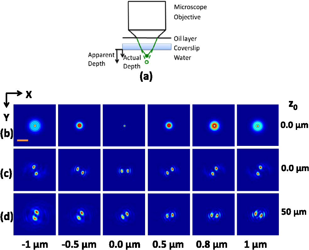 In the DH-PSF design, depth information is encoded by the angular orientation of two dominant intensity lobes in the image plane11 which rotate with the axial () position of an emitter or point source of light [Fig. 1(c)]. DH-PSFs have been used in different applications for particle tracking,12 super-resolution microscopy,13 and object ranging.14 The use of the DH-PSF in 3-D microscopy imaging coupled with single molecule imaging has provided accurate 3-D position of multiple sparse emitters from a single wide field fluorescence image.13,15 This is possible, because the center between the lobes of the DH-PSF gives the precise location of the emitter in the plane while the orientation of the lobes, when matched to a known calibration curve for the imaging system, provides the emitter’s location along the axis. In this study, the 3-D DH-PSF variability due to SA is investigated and quantified numerically using a mean-square error metric16 that reports the difference between the 3-D DH-PSF computed without SA and with different amounts of depth-induced SA. The model developed for the 3-D DH-PSF is evaluated by comparisons of simulated and experimental data. In addition, the change in the range of rotation of the DH-PSF, quantified by the calibration curve is also examined, as well as the fequency content of the DH-PSF. Because the impact of SA on the calibration curve affects the accuracy of particle localization achieved using a previously established method based on a single calibration curve,10 simulations were performed to investigate and quantify this problem under several imaging conditions with different amounts of SA over a broad range. Results previously reported about the impact of small amounts of SA17 are consistent with our results. A simple method investigated here to account for the impact of SA on particle localization, previously applied to imaging single molecules in bacteria,18 was found to be adequate only for small amounts of SA. A related approach to account for SA in a DH-PSF microscope, by calibrating axial position based upon 3-D short-time diffusion coefficients, has also been demonstrated in single particle tracking.17,19 Recently, particle position estimation based on a maximum-likelihood approach has been developed20 to provide more robust particle localization than previously achieved with the use of angle estimation and a single DH-PSF calibration curve. However, this approach is computationally expensive. The paper is organized as follows. Section 2 describes mathematical models for the DH-PSF and 3-D image formation process in the presence of SA. Methods used for the computation of the 3-D DH-PSF, the simulations, and the data-acquisition are described in Sec. 3. Results obtained from the simulations and from their comparison to experimental data are discussed in Sec. 4. The paper concludes with a summary in Sec. 5. Preliminary results from the research studies presented here have appeared in conference publications.21,22 2.Mathematical ModelsThe simulation studies presented in this paper were based on mathematical models of the DH-PSF and of image formation in a wavefront coded wide field fluorescence microscope in the presence of SA. In this section, we give a brief overview of these models. 2.1.Theoretical DH-PSFIn a wavefront coded microscope system, a phase mask with phase is placed at the back focal plane of the imaging lens which modifies the appearance of the traditional or clear aperture (CA) PSF (Fig. 2). The DH phase mask design shown by the wrapped phase values in Fig. 2(a) (leftmost image), is used to generate the DH-PSFs that encodes depth information in the spatial rotation of its main lobes [Fig. 1(c)] thereby characterizing a system with new properties. The DH phase mask was developed from the idea of wave propagation with rotating intensity distribution suggested by Piestun et al.23 which results in a high efficiency rotating PSF,24 named later as the DH-PSF because it appears as a DH along the -axis of the microscope [Fig. 2(a), rightmost image]. Fig. 2Comparison of (a) DH-PSF and (b) CA-PSF simulated images shown in , , and central cut-views from left to right, respectively. The maximum intensity projection (MIP) of the cut-view makes the double-helix appearance more evident. Images are displayed on a pixel grid using a different range of intensities in each case to allow visualization of structural details. Lens: , oil immersion. Scale bar: 3.2 μm.  Just as in the case of the CA-PSF, the DH-PSF varies with both the imaging depth (at which the microscope is focused) and the location of the light point source : where is the circular CA pupil function, is the emission wavelength of light, and are the normalized spatial frequencies, is the optical path-length error due to defocus and SA3, denotes a two-dimensional (2-D) inverse Fourier transform, is the phase of the DH mask, and the term within the braces is the modified generalized pupil function of the system. A series of 2-D PSFs at sequential forms the 3-D PSF, denoted by , and represents the 3-D image of a point source of light located at along the optical axis.2.2.Image Formation in the Presence of SAThe intensity in the 3-D image formed by a DH-based system in the presence of depth-variant imaging conditions can be written as where and represent a 3-D point in the image space and in object space , respectively; is a function representing the fluorescence concentration in the specimen; and is the depth-variant DH-PSF which changes with the actual axial location of the light point source, , with respect to the coverslip (taken to be located at ). It has been shown that it is possible to approximate Eq. (2) using a stratum-based model approximation developed previously.2 This model (reviewed here for completeness) uses a small number of depth-variant PSFs computed at different focusing depths , . These depths define nonoverlapping strata along that span the object in the object space such that . The PSF associated with the ’th stratum, for which in the object space, is determined by interpolation between two depth-variant PSFs associated with the top and bottom of each stratum, i.e., at depths and , such that: whereUsing this strata-based linear interpolation, the image of the ’th stratum can be obtained by and Eq. (2) can be approximated by the sum of all the strata images:3.Experimental MethodsThis section discusses the details for the determination of theoretical and experimental DH-PSFs under different imaging conditions that were used for the evaluation of the DH-PSF model. In addition, methodologies are developed to quantify and investigate the sensitivity of the DH-PSFs and their calibration curves to SA. Finally, details for simulations performed to investigate the use of the DH-PSF calibration curve for particle localization in the presence of SA are discussed. Simulations were performed using the COSM open source (COSMOS) software package25 and the Matlab software environment (MathWorks, Inc.). 3.1.DH-PSF ComputationThe Gibson and Lanni model3 in the COSMOS PSF module was used to compute depth variant complex-valued coherent clear aperture PSFs (CA-PSFs) for various amounts of SA (due to point sources at different depths under the coverslip either within water or glycerol) for oil-immersion lenses with various NA (1.1 to 1.3) and various wavelengths (514, 488, and 633 nm). The imaging conditions used in each case were chosen to match the imaging conditions of the experimentally determined DH-PSFs. In the case of the experimental DH-PSFs from a fabricated mask with diameter , the effective NA of the system was found to be 1.28 computed using the following formula: where is the wavelength of light, is the total number of pixels in one direction of the image, and is the pixel size.Using a Matlab script, the 2-D Fourier transform of each -plane in a 3-D complex-valued CA-PSF was computed to produce the generalized pupil function. The DH phase mask design was then applied to form a modified generalized pupil function and finally, the square magnitude of its inverse Fourier transform was computed to obtain a 2-D DH-PSF with SA [Eq. (1)]. This process was repeated for all the planes in the 3-D CA-PSF resulting in a 3-D DH-PSF. 3.2.DH-PSF Depth VariabilityTo quantify the depth variability of the DH-PSF due to SA, a normalized mean square error (NMSE) that quantifies the difference between depth-variant 3-D DH-PSFs (due to point sources at different depths) was used: where is the squared norm operation, is the 3-D PSF with SA due to a light point source located at depth below the coverslip in the presence of a RI mismatch between imaging layers, and is the 3-D PSF located at depth below the coverslip (i.e., without any SA). In general, a small NMSE value over a long range of indicates that the 3-D PSFs are similar over the depth range (i.e., the 3-D PSF of the system is insensitive to SA). For the NMSE computation, CA-PSFs and DH-PSFs were generated for light point sources in water located at depths of 0, 15, 25, 45, 75, and 100 μm below the coverslip.3.3.Experimentally Determined DH-PSFIn order to characterize the 3-D DH-PSF and its depth-variability due to SA, experimentally determined DH-PSFs were acquired from two systems (configured on an optical table at Dr. R. Piestun’s laboratory, University of Colorado, Boulder) which incorporated the DH phase mask in the back focal plane of the objective lens using a 4F system and either: (1) a fabricated phase mask;26 or (2) a spatial-light modulator implementation of the mask.27 In the first system with the fabricated mask, a magnification of , a , a wavelength of 488 nm, and an oil-immersion lens were used. DH-PSFs were imaged at two different depths from a sample with quantum dots, 100 nm in diameter (QD-050/515, Invitrogen Inc.), fixed to the coverslip and to the glass slide with a 90% glycerol solution () in between them. The experimental data consisted of images acquired at 100 different axial positions with 8 images at every axial location and a -step size of 50 nm. The images of the quantum dots fixed to the glass slide below the glycerol solution were measured at a depth of 13.5 μm below the coverslip inferred from the movement of the piezo-electric stage. In the second system (with the SLM implementation of the mask), DH-PSF images were acquired from a slide containing quantum dots (QD-525, Invitrogen Inc.) mounted in a 90% glycerol solution () using an emission wavelength of 514 nm, an oil immersion lens () with a theoretical , and an effective magnification of . The experimental data consisted of images acquired at 86 different axial positions with 8 images at every axial location and -step size of 50 nm. 3.4.Simulated Images of a 3-D Object for Particle LocalizationA computer-generated object was chosen to investigate particle localization in the presence of SA. The object comprised of three beads, with a 50 nm diameter, located at depths 0, 1.5, and 3.0 μm, respectively, within water [Fig. 3(a)]. 3-D simulated images were computed using the COSMOS Tools module for a DH system without SA [Fig. 3(b) and 3(c)] and with SA [Fig. 3(d)]. The simulated images without SA were computed using a single nonaberrant DH-PSF. To simulate depth-variant (DV) imaging due to SA, the strata-based forward-image model [Eq. (3)] was used with multiple spherically aberrant DH-PSFs defined at depths 0, 0.8, 1.6, 2.4, and 3.2 μm. Fig. 3Localization of multiple point sources using a single 2-D image from a DH-based system. central cut-view: (a) image of a three bead object with beads located at depths: 0, 1.5 and 3.0 μm; (b) image from the forward model of a DH-PSF-based system with a 3 bead structure. central cut-view from the 3-D image of this object simulated with a DH-based system computed: (c) without SA; and (d) with SA. Dashed lines in (b) and (c) show pairs of DH-PSF lobes associated with each bead. The rotation angle associated with each bead is computed and mapped to the calibration curve (e), where the rotation angle versus axial distance (defocus) from a DH-PSF without any SA is plotted. The circles in (e) indicate the locations of the three beads. Scale bars: 1.6 μm in (a); 3.2 μm in (b), and 0.8 μm in (c) and (d). Lens: oil immersion. Wavelength: 633 nm.  Particle localization in a nonaberrant system is also shown in Fig. 3(e) where the depths of the three beads in the simple object are obtained from the calibration curve through the rotation angles determined from the simulated image of the object. In the case without SA, the correct depths for the three beads (0, 1.5, and 3.0 μm, correspondingly) were determined. In the presence of SA, the observed change in the rotation angles that can be determined by the lines indicated in Fig. 3(c) and Fig. 3(d) can lead to errors. Particle localization in the presence of SA is discussed in detail in Sec. 4.2.1. 3.5.Calibration CurveThe angle subtended by the primary lobes of the DH-PSF was computed using an angle estimation algorithm28 (implemented in a Matlab) and it was plotted against axial distance to generate what is known as the calibration curve [Fig. 3(e)]. The calibration curve can be used to obtain the exact depth of point sources within an object by matching rotation angle to axial distance. Historically, the 0 deg angle associated with the best focus has been mapped to the 0 μm reference plane. However, in 3-D samples where different structures appear in focus at different axial positions, it may be more convenient to associate the 0 μm reference plane to the angle, so that other axial locations can be calculated relative to this point. We have used this convention throughout the paper. Several calibration curves were generated for different lenses under various imaging conditions. A small pixel size of 50 nm was used for the DH-PSF computation because this affects the accuracy of the calibration curve as observed in our studies. Better axial resolution gives more points for plotting the calibration curve which improves the accuracy of the calibration curve. 4.Results and DiscussionIn this section, we report results acquired from our investigations that study the impact of SA on the DH-PSF. Section 4.1.1 discusses PSF depth variability and Sec. 4.1.2 demonstrates its effect on the DH-PSF calibration curves. The use of the DH-PSF calibration curve in particle localization is investigated in the presence of SA in Sec. 4.2. Comparisons of theoretical and experimental results are shown in Sec. 4.3. Finally, the frequency content of the DH-PSF and frequency reallocation due to SA is presented in Sec. 4.4. 4.1.Effect of SA on the DH-PSFAs it is known, with increasing SA, an asymmetry in the PSF along the -axis as well as an apparent shift in the peak intensity of the CA-PSF are observed [Fig. 4(a)], resulting in the difference between the apparent and the actual location of a point light source. In the DH-PSF case, this axial shift is evident in the location of the focal plane where the two lobes are aligned along the horizontal axis, i.e., the 0 deg angle. Although this focal plane is located at when SA is not present [Fig. 1(c)] it appears at approximately in the presence of SA induced due to the point source being at a depth of 50 μm below the coverslip in water [Fig. 1(d)]. This depth variability of the 3-D DH-PSFs is clearly evident in the comparison of central cut-view images from DH-PSFs computed at different depths [Fig. 4(c)]. 4.1.1.Depth variabilityFig. 4 summarizes results that quantify the depth variability computed with Eq. (5) [Fig. 4(a)] from 3-D PSFs for a CA and a DH system at different point source depths, i.e., with a varying amount of SA [Fig. 4(b) and 4(c)]. As evident in Fig. 4(a), the NMSE for the DH-PSF changes less rapidly than the NMSE for the CA-PSFs as the axial location (depth) of the point light source in water increases, causing the SA to increase (the slight drop in the NMSE computed for the DH-PSF at depth 100 μm is an artifact due to the spread and truncation of the DH-PSF). The NMSE also suggests that for the imaging conditions simulated, the DH-PSF does not change for depths larger than . This result could be exploited in COSM that accounts for depth-variant imaging of thick samples using multiple depth-variant PSFs. As mentioned earlier, a reduction in the number of PSFs used in the computations reduces the time required to compute the fluorescence concentration in the sample. Fig. 4PSF depth variability due to SA quantified by a NMSE metric: (a) the 3-D NMSE computed for the DH-PSF and the CA-PSF. central cut-view images from 3-D PSFs of a 1.3 NA, oil lens with an effective magnification of 91.2X for: (b) a CA; and (c) an aperture with a DH mask. PSFs were computed for point light sources located at different depths (0 to 100 μm) below the coverslip in water. Scale bar: 6.4 μm.  4.1.2.Calibration curveFig. 5 summarizes the impact of both the numerical aperture (NA) of the lens and SA on the calibration curve generated for a DH-mask-based system by comparing calibration curves of DH-PSFs without SA (i.e., due to a point source at 0 μm depth under the coverslip) for lenses with a different NA [Fig. 5(a)] and calibration curves of the DH-PSFs of a single lens (with ) with increasing amounts of SA [Fig. 5(b)]. In order to show the change in the range of the DH-PSF rotation (i.e., the distance covered along as the two primary lobes rotate from to 90 deg) as the NA changes, we aligned the 3 curves shown in Fig. 5(a) at the best focus location (i.e., at the 0 deg angle). The 90 deg angle was mapped to the 0 μm axial position only for the calibration curve for in order to observe the maximum difference in the curves as the rotation angle changes in either direction from 0 deg. As it is evident in Fig. 5(a), a reduction in the NA of the lens introduces a symmetric increase in the range of rotation on either side of the 0 deg angle, i.e., the best focus. In fact, the range of rotation is proportional to where is the wavelength of light. Fig. 5Effect of NA and SA on the calibration curve of theoretically determined DH-PSFs with an effective magnification of ; oil-immersion lens. Curves for DH-PSFs with: (a) different NAs and zero SA; and (b) and different amounts of SA due to changing the location of the point source, i.e., the depth within the sample ( corresponds to the zero-SA case). Wavelength: 514 nm. RI of sample: 1.33.  However, symmetry around the 0 deg angle position is lost in the calibration curves of DH-PSFs in the presence of SA shown for the system with [Fig. 5(b)]. SA causes the range of rotation to increase only on one side of the best focus [denoted by the 0 deg. angle in Fig. 5(b)] resulting in an asymmetric calibration curve with respect to the 0 deg angle. As observed in Fig. 5(b), when the axial position moves away from the best focus towards the coverslip, the calibration curves with different amounts of SA show reasonable agreement; however, when the axial position moves deeper into the sample, the calibration curves show a significant disagreement. This is manifested by the curves converging at and completely diverging at . The change in the calibration curve due to SA impacts traditional particle localization methods that are based on the calibration curve. 4.2.Particle Localization in the Presence of SAThe accuracy of article localization based on the DH-PSF calibration curve is affected by the accuracy of the calibration curve. Figure 6(a) shows an apparent shift of the system’s best focus due to the presence of SA. For a nonaberrant system, the 0-deg angle point on the calibration curve represents the best focus of the system while for a system with SA, it represents the axial location of the circle of least confusion. In Fig. 6(b), the difference (or shift) in the axial distance evident in Fig. 6(a), is plotted versus the true axial location of the emitter for different rotation angles (which correspond to different amounts of defocus represented by the rotation angle). Fig. 6Impact of SA on the DH-PSF calibration curve. (a) Calibration curves for DH-PSFs with different amount of SA due to a point light source located at different depths within water. (b) The shift in the emitter’s axial location versus the true axial location (i.e., depth within water) of the emitter for different rotation angles (in the range of to 90 deg) for the axial location of the emitters changing from 0 to 100 μm in steps of 10 μm The inset shows a view of the observed shift for small changes in the axial locations of the emitter in the range of 0 to 3.2 μm using 5 locations from 0.0 to 3.2 μm, in steps of 0.8 μm Lens: , oil immersion. Wavelength: 633 nm. 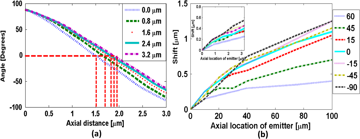 As shown in Fig. 6(b), the shift in the calibration curve changes with defocus and it is nonlinearly related with the true axial location of the emitter. For increasing SA, the apparent best focus of the emitter changes as we go deeper into the sample and thus accurate localization is not possible without the use of the calibration curve specific to the depth where the point source is located. It is interesting to note that the rate of change in the apparent location of the emitter changes through the entire range of rotation [Fig. 6(b)]. In summary, Fig. 6 shows that in the presence of SA, an error in localization occurs due to the apparent shift in the true location of a point source. In a thick 3-D sample, with multiple point sources at different depths throughout the sample, a single calibration cannot be used without incurring a particle localization error. In order to overcome this, all the calibration curves shown in Fig. 6(a) must be used. Here we propose the use of only two calibration curves: the traditional calibration curve from a nonaberrant DH-PSF and a second curve which provides a map of the apparent depth to the true depth. Such a calibration curve can be constructed from the curves in Fig. 6(a) where the depths in the legend of the figure represent the true axial location of the emitter and the apparent depth that corresponds to each of these is obtained by adding the observed shift of the “best focus” to the true depth. For small amounts of SA, this new curve is linear with a slope given by the RI ratio of the sample and the immersion medium of the lens: This relation is valid only for small amounts of SA as previously reported in a confocal microscopy study.29 We have confirmed this relation with a particle localization simulation described in the next section using the 3 bead object (discussed in Sec. 3.4). 4.2.1.Particle localization in a three-bead objectFor particle localization in the presence of SA using the angle estimation and calibration curve method, a single section image taken from a 3-D DH-system image was used [Fig. 7(a)]. The angle subtended by the two lobes, associated with each particle in the object, was estimated. As expected, these angles mapped to the traditional calibration curve of a nonaberrant DH-PSF [Fig. 7(b)] results in incorrect depths for the three beads (0, 1.7, and 3.3 μm, correspondingly). This change in precision is due to the fact that the calibration curve used does not account for the SA present in the image. This error is compensated using a second calibration curve which maps the apparent depth to the true depth [Fig. 7(c)], constructed using the axial location shift observed in 0 deg angle position of the calibrations curves with SA in Fig. 6(a) as explained above. Fig. 7Localization of particles in the presence of SA. (a) view of the forward DH-PSF image of a 3 bead object in the presence of SA. Proposed calibration curves for a system in the presence of SA: (b) rotation angle versus axial distance (defocus) from a DH-PSF without any SA (the circles indicate the apparent locations of the three beads); and (c) true axial location of emitter versus apparent depth obtained by plotting the shift observed in the best focus location from Fig. 6(a). Scale bar: 0.8 μm. Lens: oil immersion. Wavelength: 633 nm.  As the amount of SA in this study is relatively small, the apparent depth is the sum of the true depth and the shift resulting in a linear curve with a slope equal to the RI ratio in Eq. (6). However, this relation does not hold for large amounts of SA as evident by the variability of the shift in the axial position of an emitter with increasing amount of SA [Fig. 6(b)]. 4.3.Comparison of Theoretical and Experimental DH-PSFsA comparison between experimental and theoretical DH-PSFs is summarized in this section. The calibration curve for the experimental data is prepared using the same method as the one used for the simulated data described in Sec. 3.5. The first comparison study was conducted to assess the impact of SA on experimental DH-PSFs imaged from quantum dots placed on the coverslip and glass slide, respectively, as described in Sec. 3.3. Calibration curves computed from experimental DH-PSFs were compared to calibration curves from simulated DH-PSFs computed at depths 0 and 13.5 μm using the experimental imaging conditions. Four isolated quantum dots were chosen from each data set [Fig. 8(a) and 8(b)] in order to compute calibration curves for the comparison study [Fig. 8(c)]. The observed shift at the 0 deg angle between the calibration curves from the coverslip and glass slide quantum dots is determined to be 250 nm. Shift in the axial location of the beads is predicted by Eq. (6) and reinforced by the length and shift in the 0 deg angle location of the simulated DH-PSF calibration curves. The similarity in the trends observed in the simulated and experimental calibration curves of Fig. 8 is promising and validates our model. Fig. 8Effect of SA on calibration curves from experimental DH-PSFs acquired from quantum dots (QDs) in glycerol at different depths: (a) 13.5 μm; and (b) 0 μm below the coverslip. (c) Calibration curves from 4 QDs selected in each case [shown by boxes in (a) and (b)] are compared to simulated DH-PSFs with SA at a depth of 13.5 μm and without SA. Lens: 100× / 1.25 NA, oil-immersion. Scale bar: 6.4 μm.  A second study was conducted to match a theoretically determined DH-PSF to a PSF measured from quantum dots (described in Sec. 3.3) using simulations with different amounts of SA. Calibration curves and images from both the experimental and several simulated DH-PSFs are shown in Fig. 9. The asymmetrical range of rotation on either side of the “best focus” (indicating the presence of SA) covered by the experimentally determined calibration curve is determined to be from 90 to [Fig. 9(a)]. A gradual increment of the amount of SA in the [Fig. 9(c) to 9(e)] computed for the comparison study, resulted in a reasonable match between the calibration curves and the images of the measured DH-PSF [Fig. 9(b)] and a computed DH-PSF [Fig. 9(c)]. This result is quantitatively supported by Fig. 9(a), which shows that the best agreement in the calibration curves is achieved with an aberrant DH-PSF whose SA is equivalent to the amount induced by a point source located in water at a 100-μm depth below the coverslip [Fig. 9(c)]. The asymmetrical range of the theoretical DH-PSF rotation determined from the 100-μm calibration curve is from 90 to which is close to the one determined for the experimental case. Fig. 9Comparison of experimental and theoretical DH-PSFs: (a) calibration curves; and (b) to (e) cut-view images from experimental (b), and theoretically determined DH-PSFs (c) to (e) of a 91.2× / 1.3 NA oil-immersion lens. Theoretical DH-PSFs determined for a light point-source in water at a depth: (c) ; (d) ; and (e) . Scale bar: 2 μm.  Due to the noise evident in the experimental data [Fig. 9(b)], the calibration curve in Fig. 9(a) does not have the precision of the experimental calibration curves in Fig. 8(b). As expected, the large amount of SA in the system characterized in Fig. 9 (which is approximately 8 times larger than the amount of SA reported in Fig. 8) causes a reduction in the signal to noise ratio. 4.4.Effect of SA on the Frequency Content of the DH-PSFThe Fourier transform of the DH-PSF was computed to investigate its frequency content. Modulation transfer functions (MTFs) (i.e., magnitude images of computed 2-D optical transfer functions) are shown in Fig. 10 for conventional and DH-based imaging systems without SA [Fig. 10(a)] and with SA [Fig. 10(b)], respectively. The cutoff frequency for the conventional system without SA in Fig. 10 is []. Fig. 10Comparison of 2-D MTFs for a , oil-immersion lens with a 633-nm wavelength computed assuming that the light point source is in water at: (a) a 0-μm depth using a CA system (top row) and a DH system (bottom row); (b) a 2.5-μm depth (resulting in SA) using a CA system (top row) and a DH system (bottom row). Profiles along the horizontal axis through the center of each MTF for: (c) the CA system without SA; (d) the DH system without SA; (e) the CA system with SA; and (f) the DH system with SA.  As evident from this figure, the 2-D DH-MTF shows a rotation as a function of defocus (consistent with the rotation that encodes depth information in the DH-PSF) and a redistribution of frequency attenuation compared to the conventional MTFs. Except for the rotation, there is less change with defocus in the 2-D DH-MTF than in the conventional MTF. This is also evident in the profiles from the corresponding MTFs [Fig. 10(c) to 10(f)] that compare the defocused 2-D MTFs of the two systems. The oscillatory frequency attenuation of the DH-MTF [Fig. 10(d) and 10(f)] shows that the DH-MTF becomes almost zero several times along the spatial frequencies axes, and , respectively. SA attenuates the MTF frequencies as expected, but for small defocus the attenuation is less for the DH-MTF than for the MTF of the conventional system. 5.ConclusionStudies that characterize the 3-D DH-PSF and evaluate its depth-variability as a function of depth-induced SA encountered in optical sectioning microscopy of 3-D objects were presented. These studies, motivated by our interest to integrate the DH-PSF in computational optical sectioning microscopy (COSM) imaging, confirm that the DH-PSF changes less rapidly with increasing SA than the conventional PSF. This conclusion is based on the normalized mean square error result (computed between PSFs with SA and a nonaberrant PSF) and the frequency analysis of the DH-PSF presented. This is a promising result for the use of the DH-PSF with algorithms that use multiple depth-variant PSFs in COSM. The use of fewer PSFs in the computations makes these approaches more practical for biological use. The impact of SA on the frequency content of the DH-PSF is shown to be different from the impact it has on the conventional PSF frequency content. The modulation transfer function computed from the DH-PSF (DH-MTF) shows extended depth of field that preserves spatial frequencies with defocus and SA. The frequency rearranging observed in the DH-MTF in the presence of SA seems favorable for COSM imaging of thick samples. Our detailed study of the aberrant DH-PSF elucidated the impact of SA on particle localization accuracy when a calibration curve from a nonaberrant DH-PSF is used. The rate of rotation observed in the DH-PSF was shown to slow down with SA. This causes an extension in the range of rotation and results in asymmetric rotation ranges as the focus is moved in opposite directions. Theoretical DH-PSFs compared to experimental ones show the same trend when an appropriate amount of SA is incorporated in the theoretical DH-PSF. In the presence of SA, particle localization accuracy using the traditional DH-PSF calibration curve can be improved by using a second calibration curve to account for the axial shift due to SA. Although the PSF model used in this investigation includes apodisation effects, it does not include vectorial effects which can affect the appearance of the DH-PSF and consequently its range of rotation for the high NA system modeled here. However, we expect the use of a more accurate vectorial30 model would not change the observed trend. Theoretical and experimental studies performed to characterize the DH-PSF under varying imaging conditions show reasonable agreement between theoretical and experimental DH-PSFs, suggesting that our model can predict the main features of the data. Thus, the DH-PSF model evaluated in these studies can be used in the model-based algorithms previously developed for COSM. AcknowledgmentsWe thankfully acknowledge our collaborator Dr. R. Piestun and his students Dr. S. Quirin, A. Barsic, and G. Grover at the University of Colorado, Boulder, for providing the quantum dot data, example Matlab code for the DH-PSF computation and angle estimation, and for useful discussions. We are very grateful to the anonymous reviewers and to Dr. S. V. King for their useful comments and suggestions. This work was supported by the National Science Foundation (NSF CAREER award DBI-0844682, PI: C. Preza; and NSF Collaborative IDBR awards DBI-0852847, PI: C. Preza; and DBI-0852885, PI: R. Piestun) and the Herff College of Engineering, at the University of Memphis (Graduate Herff fellowship to S. Ghosh). ReferencesD. A. Agard,
“Optical sectioning microscopy,”
Annu. Rev. Biophys. Bioeng., 13 191
–219
(1984). http://dx.doi.org/10.1146/annurev.bb.13.060184.001203 ABPBBK 0084-6589 Google Scholar
C. PrezaJ.-A. Conchello,
“Depth-variant maximum-likelihood restoration for three-dimensional fluorescence microscopy,”
J. Opt. Soc. Am. A, 21
(9), 1593
–1601
(2004). http://dx.doi.org/10.1364/JOSAA.21.001593 JOAOD6 0740-3232 Google Scholar
S. F. GibsonF. Lanni,
“Experimental test of an analytical model of aberration in an oil-immersion objective lens used in 3-dimensional light-microscopy,”
J. Opt. Soc. Am. A, 9
(1), 154
–166
(1992). http://dx.doi.org/10.1364/JOSAA.9.000154 JOAOD6 0740-3232 Google Scholar
C. PrezaV. Myneni,
“Quantitative depth-variant imaging for fluorescence microscopy using the COSMOS software package,”
Proc. SPIE, 7570 757003
(2010). http://dx.doi.org/10.1117/12.840688 PSISDG 0277-786X Google Scholar
S. YuanC. Preza,
“Point-spread function engineering to reduce the impact of spherical aberration on 3D computational fluorescence microscopy imaging,”
Opt. Express, 19
(23), 23298
–23314
(2011). http://dx.doi.org/10.1364/OE.19.023298 OPEXFF 1094-4087 Google Scholar
M. Arigovindanet al.,
“A parallel product-convolution approach for representing depth varying point spread functions in 3D widefield microscopy based on principal component analysis,”
Opt. Express, 18
(7), 6461
–6476
(2010). http://dx.doi.org/10.1364/OE.18.006461 OPEXFF 1094-4087 Google Scholar
G. Saavedraet al.,
“Reduction of spherical-aberration impact in microscopy by wavefront coding,”
Opt. Express, 17
(16), 13810
–13818
(2009). http://dx.doi.org/10.1364/OE.17.013810 OPEXFF 1094-4087 Google Scholar
E. R. DowskiW. T. Cathey,
“Extended depth of field through wave-front coding,”
Appl. Opt., 34
(11), 1859
–1866
(1995). http://dx.doi.org/10.1364/AO.34.001859 APOPAI 0003-6935 Google Scholar
W. T. CatheyE. R. Dowski,
“New paradigm for imaging systems,”
Appl. Optics, 41
(29), 6080
–6092
(2002). http://dx.doi.org/10.1364/AO.41.006080 APOPAI 0003-6935 Google Scholar
S. R. P. PavaniA. GreengardR. Piestun,
“Three-dimensional localization with nanometer accuracy using a detector-limited double-helix point spread function system,”
Appl. Phys. Lett., 95
(2), 021103
(2009). http://dx.doi.org/10.1063/1.3158923 APPLAB 0003-6951 Google Scholar
A. GreengardY. Y. SchechnerR. Piestun,
“Depth from diffracted rotation,”
Opt. Lett., 31
(2), 181
–183
(2006). http://dx.doi.org/10.1364/OL.31.000181 OPLEDP 0146-9592 Google Scholar
S. R. P. PavaniR. Piestun,
“Three dimensional tracking of fluorescent microparticles using a photon-limited double-helix response system,”
Opt. Express, 16
(26), 22048
–22057
(2008). http://dx.doi.org/10.1364/OE.16.022048 OPEXFF 1094-4087 Google Scholar
S. R. P. Pavaniet al.,
“Three-dimensional, single-molecule fluorescence imaging beyond the diffraction limit by using a double-helix point spread function,”
Proc. Natl. Acad. Sci. U.S.A., 106
(9), 2995
–2999
(2009). http://dx.doi.org/10.1073/pnas.0900245106 PNASA6 0027-8424 Google Scholar
S. QuirinS. R. P. PavaniR. Piestun,
“Broadband three-dimensional imaging using a double-helix point spread function,”
in Computational Optical Sensing and Imaging,
(2009). Google Scholar
S. R. P. PavaniR. Piestun,
“3-D fluorescent particle tracking with nanometer scale accuracies using a double-helix point spread function,”
in Lasers and Electro-Optics/International Quantum Electronics Conference,
(2009). Google Scholar
S. YuanC. Preza,
“Point-spread function engineering to reduce the impact of spherical aberration on 3D computational fluorescence microscopy imaging,”
Opt. Express, 19
(23), 23298
–23314
(2011). http://dx.doi.org/10.1364/OE.19.023298 OPEXFF 1094-4087 Google Scholar
M. A. Thompsonet al.,
“Three-dimensional tracking of single mRNA particles in Saccharomyces cerevisiae using a double-helix point spread function,”
Proc. Natl. Acad. Sci. U.S.A., 107
(42), 17864
–17871
(2010). http://dx.doi.org/10.1073/pnas.1012868107 PNASA6 0027-8424 Google Scholar
M. D. Lewet al.,
“Three-dimensional superresolution colocalization of intracellular protein superstructures and the cell surface in live Caulobacter crescentus,”
Proc. Natl. Acad. Sci. U.S.A., 108
(46), E1102
–E1110
(2011). http://dx.doi.org/10.1073/pnas.1114444108 PNASA6 0027-8424 Google Scholar
J. M. Casolariet al.,
“Widespread mRNA association with cytoskeletal motor proteins and identification and dynamics of myosin-associated mRNAs in S. cerevisiae,”
PLoS ONE, 7
(2), e31912
(2012). http://dx.doi.org/10.1371/journal.pone.0031912 1932-6203 Google Scholar
S. QuirinS. R. PavaniR. Piestun,
“Optimal 3D single-molecule localization for superresolution microscopy with aberrations and engineered point spread functions,”
PNAS, 109
(3), 675
–679
(2012). http://dx.doi.org/10.1073/pnas.1109011108 PNASA6 0027-8424 Google Scholar
S. Ghoshet al.,
“Effect of double-helix point-spread functions on 3D imaging in the presence of spherical aberrations,”
Proc. SPIE, 7904 79041D
(2011). http://dx.doi.org/10.1117/12.874111 PSISDG 0277-786X Google Scholar
S. Ghoshet al.,
“Computational imaging for fluorescence microscopy using double helix PSF engineering,”
Proc. SPIE, 8227 82270F
(2012). http://dx.doi.org/10.1117/12.909757 PSISDG 0277-786X Google Scholar
R. PiestunY. Y. SchechnerJ. Shamir,
“Propagation-invariant wave field with finite energy,”
J. Opt. Soc. Am., 17
(2), 294
–303
(2000). http://dx.doi.org/10.1364/JOSAA.17.000294 JOSAAH 0030-3941 Google Scholar
S. R. P. PavaniR. Piestun,
“High-efficiency rotating point spread functions,”
Opt. Exp., 16
(5), 3484
–3489
(2008). http://dx.doi.org/10.1364/OE.16.003484 OPEXFF 1094-4087 Google Scholar
G. SharmaS. R. P. PavaniR. Piestun,
“Optimization of double-helix point spread function for photon-limited 3D imaging systems,”
in Computational Optical Sensing and Imaging,
(2009). Google Scholar
S. R. P. PavaniR. Piestun,
“Three dimensional tracking of fluorescent microparticles using a photon-limited double-helix response system,”
Opt. Express, 16 22048
–22057
(2008). http://dx.doi.org/10.1364/OE.16.022048 OPEXFF 1094-4087 Google Scholar
S. A. Quirin,
“Quantitative optical imaging and sensing by joint design of point spread functions and estimation algorithms,”
1
–220 University of Colorado, Boulder
(2012). Google Scholar
A. EgnerS. W. Hell,
“Aberrations in confocal and multi-photon fluorescence microscopy induced by refractive index mismatch,”
404
–413 Springer Science and Business Media, New York
(2006). Google Scholar
O. Haeberle,
“Focusing of light through a stratified medium: a practical approach for computing microscope point spread functions. Part I: Conventional microscopy,”
Opt. Commun., 216
(1–3), 55
–63
(2003). http://dx.doi.org/10.1016/S0030-4018(02)02282-4 OPCOB8 0030-4018 Google Scholar
|


