Improvements in speckle tracking algorithms for vibrational analysis using optical coherence tomography

Prashanth Raghavendra Prasad; Shanti Bhattacharya

doi:10.1117/1.JBO.18.4.046007

8 April 2013 Improvements in speckle tracking algorithms for vibrational analysis using optical coherence tomography

Prashanth Raghavendra Prasad, Shanti Bhattacharya

Author Affiliations +

Journal of Biomedical Optics, Vol. 18, Issue 4, 046007 (April 2013). https://doi.org/10.1117/1.JBO.18.4.046007

Abstract

We report on improvements in speckle tracking algorithms for analyzing subsurface vibrations using an optical coherence tomography system. Our technique uses axial deconvolution and linear interpolation of depth scans before using cross-correlation-based speckle tracking. We applied this method on M-mode images of a test sample and on wrist pulses to perform depth-resolved measurements of displacement, velocity, and frequencies of vibrations. Speckle pattern displacements and features spanning 0.5 pixels were tracked clearly. Extension of this technique to two dimensions can provide improved performance in the field of optical coherence elastography.

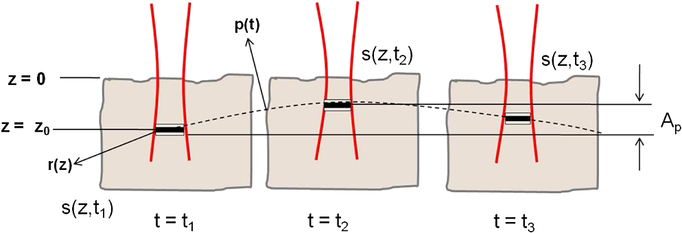
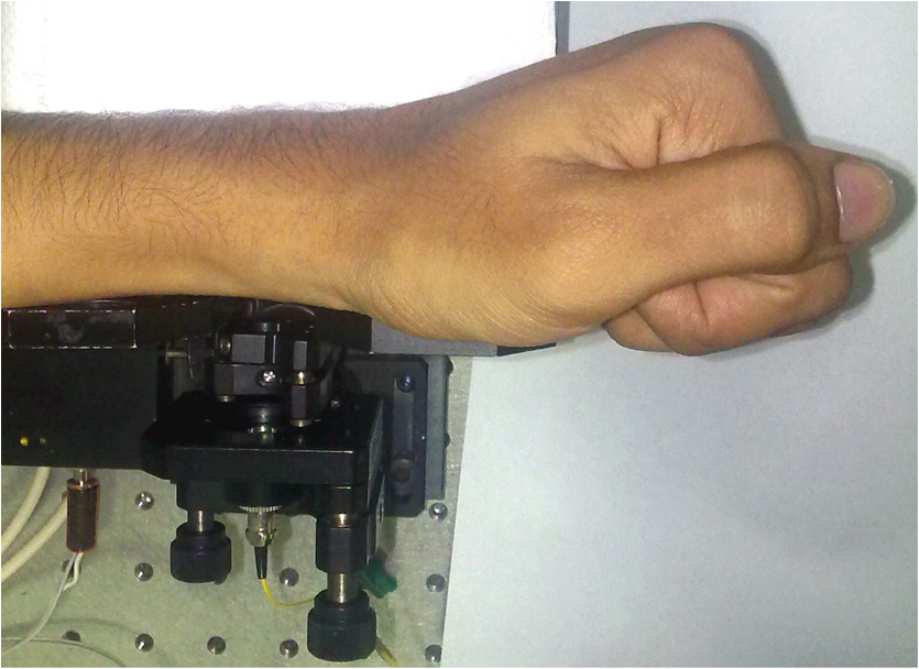
1. Introduction

Detection and analysis of motion in biological tissues is of great importance in the fields of medicine and developmental biology. A considerable amount of research effort has been applied in probing and analyzing vibration patterns in organs like the vocal tract, inner ear, heart tubes, etc.¹^–³ The bio-elastic properties of skin have been studied by analyzing its response to externally applied vibrations.⁴ Optical coherence tomography (OCT), with its noncontact and noninvasive depth resolved imaging capabilities has emerged as a powerful technique for imaging biological tissues.⁵^,⁶ It offers micrometer resolution and depth of penetration of 2 to 3 mm in scattering samples. It has been used previously to image and analyze subsurface motion and vibrations in biological tissues. Schmitt demonstrated the use of OCT for measuring elastic properties of tissues, giving birth to optical coherence elastography (OCE) in 1998.⁷ That work involved tracking of movements of specific tissue portions between images, using speckle tracking. More recently, many researchers have used OCT to analyze subsurface vibrations in samples⁸^,⁹ by tracking displacements of sample segments between successive depth scans acquired at a fixed position on the sample surface (also called M-mode scan). In OCT, displacement of sample segments can be measured using either speckle tracking or phase tracking methods. Speckle tracking involves finding the displacement vector of a group of image pixels forming a pattern. Variants of this method include peak tracking, edge tracking and cross-correlation-based tracking. Phase tracking involves detecting the shift in phase at desired locations between successive OCT scans. The displacement vector can subsequently be found by dividing the phase shift by the wave propagation constant for the sample medium. A variant of the phase tracking method, called Doppler OCT measures the frequency shift due to the motion of sample segments. The phase tracking algorithm¹⁰^,¹¹ is capable of detecting nanometer scale sample displacements and velocities, with high dynamic range. However, it has the drawback of phase aliasing.¹² In human vocal cords, small scale displacements have amplitudes of few hundreds of micrometers and peak velocities exceeding one metre/second.¹³ Phase tracking cannot detect such high velocity vibrations using most of the commercially available OCT systems except possibly the latest high speed megahertz line scan rate OCT, involving expensive data acquisition and signal processing hardware.¹⁴ Also in cases where the image signal to noise ratio (SNR) is low, traditional phase resolved tracking methods underestimate the displacement, leading to tracking errors. Kennedy et al.¹⁵ have overcome this drawback by using joint spectral-time domain OCE technique, which also uses phase information for tracking displacements.

Speckle tracking is an alternative method for tracking large displacements, but with reduced accuracy. Several research groups have attempted to improve the accuracy of speckle tracking methods using OCT. Speckle tracking based on velocity estimation was proposed in 2002¹⁶^,¹⁷ to track motion along one dimension. This method used maximum likelihood solution methods to predict speckle velocity at subpixel resolutions. Kirkpatrick et al. extended this method to two dimensions in their work.¹⁸ While it was claimed that the method could measure displacements as low as 0.1 pixels, it was also shown that the method performed optimally up to speckle motions of $0.8 pixels / record$ , beyond which cross-correlation methods provide better performance. To overcome this disadvantage, the authors proposed the use of a variant of phase tracking method, called tissue Doppler optical coherence elastography (tDOCE) for tracking larger displacements.

In this article, we demonstrate improvements in cross-correlation-based speckle tracking method for tracking vibrations in a sample at subpixel resolution. Our objective was to extend the capability of cross correlation based speckle tracking to detect subpixel movements without sacrificing accuracy at larger multipixel displacements. Specifically, we have used deconvolution and interpolation processes prior to performing cross-correlation for determining speckle movements in M-mode OCT images. Deconvolution methods have previously been used in OCT to improve axial resolution by making use of the coherence function of the broadband source.¹⁹^,²⁰ Image interpolation methods have featured previously in ultrasound imaging for enhancing the accuracy of motion tracking.²¹ We report the results of tracking displacements in the vibrations of wrist pulse. Using the combination of deconvolution and interpolation we have achieved tracking resolutions of about 0.5 pixel when the sample region has a total displacement over twenty pixels.

2. Methods

2.1.

Speckle Tracking in One Dimension

Consider a sample section $s (z, t)$ lying under the probing system as shown in Fig. 1. The structure of the sample section varies with depth and time, since the sample is under oscillation. A small subsection $r (z)$ of $s (z, t)$ , lying at a depth and $z_{0}$ oscillating with an amplitude $A_{p}$ is considered for analysis. It is assumed that the structure and reflectivity profile of $r (z)$ do not change with time, due to its small size. In Fig. 1, $p (t)$ denotes the time dependent position of the subsection.

Fig. 1

Illustration showing the movement of the sample feature $r (z)$ under the sample surface.

The M-mode scan of the sample section $S$ , taken at any time instant $t$ can be expressed as the convolution:

Eq. (1)

I (z, t) = \exp (- γ z) \int s (z^{'}, t) c (z - z^{'}) d z^{'}

Eq. (2)

= [c (z) * s (z, t)] \exp (- γ z) .

Here

c (z)

is the axial coherence function of the OCT system. The exponential factor, containing the mean scattering co-efficient (

γ

), accounts for the depth dependent attenuation of light intensity in the image.⁷ Since the sample feature

r (z)

vibrates at a mean depth of

z_{0}

, with an amplitude

A_{p}

, the reference position is taken to be

z_{0}

. Further, the exponential decay of intensity is ignored over small thickness of

r (z)

. At time instant

t_{1}

, the segment profile is given by

I_{z_{0}} (z, t_{1})

.

Eq. (3)

I_{z_{0}} (z, t_{1}) = c (z) * r (z) = I_{1} (z) (say) .

At another instant

t_{2}

, the segment would have moved some distance

δ z

along the depth axis, giving the profile

I_{z_{0}} (z, t_{2})

. Under the assumption that the depth profile of

r (z)

remains the same between time instants

t_{1}

and

t_{2}

, we may use the property of shift invariance to express

I_{z_{0}} (z, t_{2})

in terms of

I_{1} (z)

as

Eq. (4)

I_{z_{0}} (z, t_{2}) = c (z) * r (z - Δ z)

Eq. (5)

= I_{1} (z - Δ z) = I_{2} (z) (say) .

Here,

δ (•)

is the shift operator. Next, the cross correlation between

I_{1} (z)

and

I_{2} (z)

is computed.

Eq. (6)

C_{z_{0}} (z) = \int_{- l}^{l} I_{1} (u) I_{2} (u - z) d u = \int_{- l}^{l} I_{1} (u) I_{1} (u - z - Δ z) d u .

Here,

l = A_{p} / 2

defines the limits of integration. The differential displacement can be extracted as

Eq. (7)

Δ z = \underset{z}{\arg \max} [C_{z_{0}} (z)] .

The

\arg \max (•)

operator indicates the value of the argument

z

, for which

C_{z_{0}} (z)

is maximum. If

p (t_{0}) = z_{0}

is taken as the reference position, then, the position of the subsection

r (z)

at any time instant

t_{i}

may be computed by adding the differential displacements taken at time

t

as

Eq. (8)

p (t_{i}) = \int_{0}^{t_{i}} Δ z (t) d t,

where

d t

is the differential time between two depth scans. The velocity may be computed by taking the time differential of

p (t)

. That is,

Eq. (9)

v (t) = \frac{d p (t)}{d t} .

Thus, the displacement and velocity profiles of vibrations under the sample surface may be determined.

The mathematical analysis described so far assumes that the depth scans are continuous functions of depth axis $z$ . Also, it was assumed that the time interval between two depth scans was small. In practice, the M-mode image is discrete along both depth and time axes, due to the finite number of pixel elements in the detector and finite time interval between two successive depth scans. Discretization along the axial direction limits the minimum displacement of the sample subsection that can be measured to the axial distance spanned by one pixel in the M-mode scan. The next section describes the use of deconvolution and interpolation methods to allow tracking of subpixel motion.

2.2.

Axial Deconvolution and Linear Interpolation

A two-step procedure is employed for improving the tracking accuracy of the cross-correlation-based speckle tracking method. First, the sharpness of image features (or equivalently the axial resolution) is improved by deconvolving the depth scans using the coherence function of the system. The axial resolution of OCT images is determined by the coherence properties of the broadband source used for illuminating the interferometer. Most commonly, the coherence length ( $l_{c}$ ) of the source is used as the axial resolution of the image. The Lucy-Richardson algorithm was used for deconvolving the depth scans of M-mode images. The algorithm has the expression:²²

Eq. (10)

e_{k + 1} (z) = e_{k} (z) [h (- z) * \frac{g (z)}{h (z) * e_{k} (z)}] .

Here

e_{k}

is the

k

’th iteration of the deconvolved axial scan,

g (z)

is the original axial scan, and

h (z)

is the point spread function, which is the coherence function of the broadband source in this case.

Following this, linear interpolation was performed on depth scan segments for enabling smoother cross-correlation. It is assumed that the velocity of the sample section $r (z)$ is constant over the short sampling interval $T$ because of which the position of $r (z)$ varies linearly within the sampling interval. Thus, linear interpolation may be used to estimate the position of the sample section between the sampling interval. If $x (n)$ is a depth scan in the M-mode image, the interpolated value $y (k)$ between the $i$ ’th and $i + 1$ ’th pixels is

Eq. (11)

y (k) = x (i) + [x (i + 1) - x (i)] (k - i) i < k < i + 1 .

In theory, tracking precision can be improved arbitrarily by having large number of interpolant points between two base intensity points in $x (n)$ . However, ambient noise in the image sets an upper limit to the tracking accuracy. One possible criterion is to ensure that the difference between successive interpolant points be greater than the noise variance in the image region. That is, if $σ_{n}$ is the noise variance in the image region, then

Eq. (12)

y (k + 1) - y (k) > σ_{n} .

Figure 2 illustrates the effect of interpolation of depth scans in the segments. A sample feature moves through a distance less than a pixel between time instants $t_{1}$ and $t_{2}$ , which is the time interval between successive depth scans ( $T$ ). Before interpolation [Fig. 2(b)] the subpixel movement cannot be resolved since the minimum displacement that can be detected is one pixel. Under the assumption that the velocity of motion of the sample feature is constant within the depth scan interval $T$ , it is possible to estimate intensity values between two pixels using linear interpolation, as shown in Fig. 2(c). Now, the subpixel movement is represented by several points, enabling the cross correlation method to track the same. In Fig. 2(c), four intensity values are estimated between two successive pixels. In the experiments, 10 points were estimated between two pixels to improve tracking accuracy.

Fig. 2

Illustration showing the interpolation process. (a) Depth scans taken at different time instants. (b) Measured depth before interpolation. (c) Measured depth after interpolation. The curve in (b) and (c) shows the actual movement of the sample. The longer horizontal lines (red in online version) indicate the measured values before interpolation and the short horizontal lines (green in online version) show the interpolated values.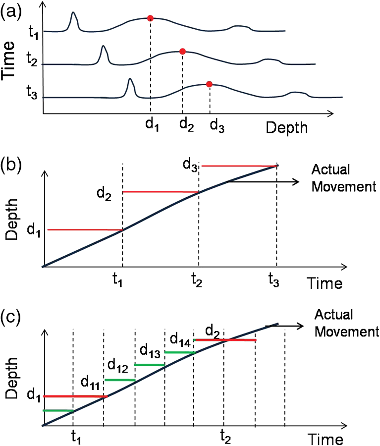

3. Results

A spectral domain OCT system (Fig. 3) with a center wavelength of 1565 nm and a bandwidth of 74 nm was used in our experiments, giving an axial resolution of 16.5 μm in air. In the sample arm of the Michelson interferometer, a 10 mm focal length lens was used to focus a collimated beam of 0.9 mm diameter, providing a beam spot of 22 μm diameter, which is the lateral resolution of the system. An indium gallium arsenide (InGaAs)-based spectrometer having a 512 pixel line camera was used at the detector arm. The line scan rate was set to 200 Hz for acquisition of M-mode images. The system sensitivity was estimated to be about 88 dB using the procedure described in Ref. 23. It should be noted that the relatively low sensitivity obtained was a result of the spectrometer used to capture the interference spectra, and is not indicative of the ability of the algorithm. The spectrometer was a USB-based developer module, with an uncooled detector. However, its sensitivity was high enough to achieve reliable performance of the tracking algorithm, as seen in the results. The maximum imaging depth was computed to be about 3.68 mm and the 6 dB SNR drop-off distance was estimated to be about 3.25 mm.

Fig. 3

Block diagram of the spectral domain OCT system used for experiments.

A custom built test sample consisting of static and vibrating structures was used to test the vibrational analysis method discussed in the previous section. Image processing was carried out using MATLAB (MathWorks) software.

3.1.

Validation of Speckle Tracking Method Using a Test Sample

Ten layers of pressure sensitive adhesive tape were adhered one over another to form a stack. A CD-pickup head with a gold-coated reflector attached to its front end was held in position behind the tape stack. This vibrating structure along with the static layers was used as a test sample. The pickup head could be vibrated by applying electrical excitation. The sample beam of the OCT system was incident on the tape stack as shown in Fig. 4. In this arrangement, the tape stack formed a static reflecting structure and the gold-coated reflector on the pickup head formed the vibrating structure. The mirror (gold-coated reflector) can be considered to be an extremely thin reflector so that its intensity profile can be represented by the impulse function $δ (z)$ . In that case, according to Eq. (3), the intensity profile of the mirror in the depth scan is nothing but the coherence function of the broadband source itself. In general, the coherence function decays gradually around its central peak and hence occupies more than one pixel in the depth scan. This allows one to track the displacements of the mirror using cross-correlation. The characterization of the pickup head had been carried out earlier,²⁴ using a Michelson interferometer with a low coherence source. The characterization method is explained briefly here for the sake of continuity. One of the reflectors of the interferometer was replaced with a mirror attached to the the pickup head to be characterized. The path length difference between the arms could therefore, be varied by actuating the pickup head. The output of the interferometer was captured on a photodetector (PD) and viewed on an oscilloscope. The coherence length of the source was calculated using the spectral width of the source obtained from optical spectrum analyzer measurements. Since the source used was a low coherence one, fringes were observed only when the path length was less than the coherence length of the source, as seen in Fig. 5(a). The initial calibration consisted of estimating the mirror velocity for driving signals of different amplitudes and frequencies. In each case, the time taken by the mirror to traverse the coherence length was obtained from the oscilloscope trace. The second step was to use the calculated values of velocity to estimate the distance travelled by the mirror for a $Δ t$ corresponding to the time interval between two peaks of the coherence envelopes as seen in Fig. 5(b). The number of coherence envelopes seen will vary depending on the frequency of the mirror. The calibration was completed by calculated the displacement of the pick-up to driving signals of different frequencies but the same peak voltage and driving signals of different peak voltages but the same frequency. This is shown in Fig. 5(c) and 5(d), respectively. Based on the calibration, it was decided to operate the pick-up at a low peak voltage of 30 mV and at frequencies below 19 Hz. The former was done as the pick-up was meant to create only small displacements and the latter was chosen so as to avoid the resonance frequency.

Fig. 4

Test sample structure for validation of the displacement tracking algorithm.

Fig. 5

Characterization of the CD-pickup head. (a) Output of a Michelson Interferometer with a low coherence input source. The ratio of the coherence length to the time difference between the points where the amplitude of the interference envelope falls to $1 / e$ of the peak value is taken as the velocity of the mirror. This measurement was repeated a number of times and the average value was used as the mirror velocity. Note that the PD responds to the intensity of the incident light beam, but this figure plots the amplitude of the voltage response of the PD with respect to time. (b) The velocity of the mirror attached to the pick-up head depends on the amplitude and frequency of the voltage applied to it. In turn, the number of low coherence envelopes seen in a certain time interval will depend on the velocity of the mirror. If the velocity of the mirror is known, the distance traversed by the mirror in an interval $Δ t$ , i.e., its displacement can be calculated. (c) The displacement of the mirror was found to increase linearly with increase in applied voltage at a frequency of 15 Hz. This behavior was true as long as the voltage did not exceed 2 V. The markers indicate values obtained from measurements and the straight line is the linear fit to these points. (d) A maximum voltage of 1.5 V was applied to the mirror and its behavior at different frequencies was observed. The resonance frequency of the mirror was found to occur close to 19 Hz.

Figure 6 shows the vibrational analysis for the M-mode scan of the test sample shown in Fig. 4. The displacement tracking algorithm was applied on two segments of the M-mode scan, marked as regions 1 and 2.

Fig. 6

Vibration analysis using the M-mode scan of the pickup head. Segments 1 and 2 are indicated by the white vertical bars in (a). In the profiles, the segments 1 and 2 are denoted by continuous and dotted lines, respectively. The displacement profile and instantaneous velocity are shown respectively in (b) and (c). The frequency components of vibration are shown in (d).

Both segments span 21 pixels in depth, so that the peak to peak displacement of the vibrating mirror is covered. In Fig. 6(b), segment 1 (continuous) shows zero displacement throughout the time span since the tape layers are stationary. Based on the CD-pickup head characterization, the peak-to-peak displacement was estimated to be about 214 μm. The excitation was a combination of two frequencies (14.5 Hz-320 mV and 17 Hz-196 mV). In Fig. 6(b), the peak-peak displacement of segment 2 between 208 and 220 μm, giving an error of less than half a pixel from the mean estimated value. The velocity variation is also a combination of sinusoids since the differential of sinusoid displacement is a phase shifted and scaled sinusoid, and in this case, has a peak value of about $10 mm / s$ . The frequency components of the vibration shown in Fig. 6(d), measured to be 14.6 and 17 Hz, match closely with the applied frequencies of 14.5 and 17 Hz.

In another experiment, the pickup head was excited with a single sinusoidal frequency of 14.5 Hz of 30 mV amplitude. The displacement curves are shown in Fig. 7.

Fig. 7

Response of pickup head for 30 mV excitation amplitude at 14.5 Hz. The displacement tracking method was applied at region 1.

Based on the characterization of the pickup head, the displacement amplitude was estimated to be about 3.5 μm. The measured waveform is a sinusoid with amplitudes varying from 3.8 to 4.6 μm. In free space, each pixel of the image spans 16.5 μm. Since the measured amplitude of the mirror is around 4.2 μm with a deviation of about 0.8 μm, we estimate conservatively that the minimum tracking accuracy of our method to be at least 0.5 pixels (8.25 μm in free space).

3.2.

Subsurface Analysis of Wrist Pulse Oscillations

Once validated using the test sample structure, the displacement tracking method was applied to analyze wrist pulse oscillations at the radial artery. Wrist pulse was chosen since its pulse waveform characteristics are well studied by other methods enabling us to compare our results. Pulse measurements were undertaken on healthy volunteers after informed consent. An in-house developed mount was used to hold the wrist in place. This was achieved by having a post, which the user could grasp with her hand, as seen in Fig. 8. By having the hand fixed in this way, motion artifacts could be reduced.

Fig. 8

Custom-built arrangement used for acquiring M-mode scans of wrist pulse.

Figure 9 shows the results of vibration analysis on wrist pulse. The M-mode scan of wrist pulse at the radial artery is shown in Fig. 9(a). The displacement tracking method was applied on two segments at different depths—shown as regions 1 and 2 in Fig. 9. Both regions correspond to portions of the sample that are moving. Region 1 is about 225 μm (20 pixels) deep starting from the surface and region 2 spans 225 μm further. This is after considering the improvement in the axial resolution (from 16.5 to 11.6 μm) due to the mean refractive index (1.42) of skin.²⁵ It is seen in Fig. 9 that the structure of the segment (and the layers within it) under vibration is maintained well throughout the scan duration. Thus, the assumption of shift variance of $r (z)$ in Eq. (4) is valid.

Fig. 9

Displacement profiles extracted from the wrist pulse measurements. (a) Wrist pulse, (b) zoomed profile of region 1, (c) zoomed profile of region 2, (d) displacement in region 1, and (e) displacement in region 2.

The mean SNRs were measured to be, respectively 41.8 dB and 38.9 dB using the method described in Ref. 26. In the figure, displacement of the subsection in region 1 is tracked with reasonable accuracy. In region 2, the algorithm fails to track the displacement accurately, possibly due to poorer SNR, compared to region 1. Figure 10 shows the variation of SNR across the regions 1 and 2. In region 1, the inclusion of dark space for averaging results in a low value for mean SNR. In contrast, region 2 has lower mean SNR even when the sample features cover the entire image.

Fig. 10

SNR map for regions 1 and 2 of wrist pulse vibration measurement.

Figure 11 shows the M-mode scan of wrist pulse after deconvolution. Zoomed in parts of the two interpolated segments, region 1 and region 2 are shown in Fig. 11(b) and 11(c). Their displacement profiles are shown in Fig. 12(a) and 12(b), respectively.

Fig. 11

(a) M-mode scan of wrist pulse, (b) zoomed image of region 1, and (c) zoomed image of region 2.

Fig. 12

Displacement profiles of wrist pulse oscillations (a) displacement profile in region 1, (b) displacement profile in region 2. In the plot, $p q = 17 μ m$ $p r = 40 μ m$ and $m n = 7 μ m$ . $s$ : systolic peak, and (d) diastolic peak w: reflected wave.

In this case, fine variations in radial artery pulse movements are apparent and compare well with the same acquired by other researchers using methods other than OCT.²⁷^,²⁸ Although individual pulse patterns differ slightly, systolic, diastolic and the reflected components of the pulse waveform can be discerned. The peak-to-peak amplitude of oscillation varies between 40 to 55 μm (4 to 5 pixels before interpolation), taking into account the mean refractive index (1.42) of skin.²⁵ The height difference between the systolic and diastolic wave peaks was measured to be around 17 μm or about 1.5 pixels. The reflected wave component,²⁹ spanned 7 μm in height, or about 0.6 pixels. We deduce that the system is capable of measuring displacements of minimum 0.5 pixels, considering the subpixel height difference between the systolic and the diastolic peaks.

The velocity variation profile and the frequency components of wrist pulse are shown in Fig. 13 for both regions 1 and 2. The velocity peaks coincide with the start of the pulse oscillations. The fundamental frequency peak occurs at 1.4 Hz. Apart from deconvolution and interpolation, elementary signal processing was used to remove unavoidable artifacts that occurred during experiments. High pass filtering was used to suppress arbitrary motion artifacts due to the stretching/relaxation of wrist skin surface. Also, random high frequency noise occurring in the displacement and velocity data was minimized by using running average of 10 and 3 points, respectively. A comparison was made between the pulse rates determined using the method discussed above and the palpatory method wherein the pulse measurements were taken by a medical professional. The fundamental frequency of pulse oscillation determined using the Fourier components was multiplied by 60, in order to obtain the pulse rate in beats per minute. Four healthy subjects volunteered for the experiments. Table 1 shows the comparison. It is seen that the measurements made with the OCT system are in good agreement with those obtained from the palpatory method.

Fig. 13

Velocity profile and frequency components for pulse vibrations. (a) Velocity profile. (b) Frequency components.

Table 1

Radial arterial pulse rates in beats/minute measured by the SDOCT system and a medical professional.

Subject	SDOCT system	Medical professional
1	78	80
2	72	70
3	78	76
4	84	80

4. Discussion

We have reported an improved speckle tracking method for detection and analysis of subsurface vibrations in samples using OCT. Application of axial deconvolution and interpolation methods to OCT images, prior to speckle tracking, is shown to deliver better performance of the tracking algorithm. To our knowledge, we have demonstrated improvements in speckle tracking methods in OCT by using deconvolution and interpolation, for the first time. The smallest displacement tracked in our experiments is 0.5 pixel. While this is larger than the resolution (0.1 pixel) claimed previously,¹⁷ the improved cross-correlation method can track larger multipixel displacements without compromising accuracy. This is evident in the displacement profile of vibration of the cd pickup head. The difference between the predicted and measured displacements of the cd-pickup head, 214 μm and 208 to 220 μm is less than 0.5 pixel over a total displacement of 21 pixels. At present, we could not test the interpolation method for smaller displacements since the pickup head was unreliable for excitations below 30 mV, corresponding to a mean displacement of 6 μm, in Fig. 7. However, in other research areas like particle image velocimetry interpolation-based speckle tracking methods have yielded tracking accuracies of up to 0.01 pixels.³⁰ The execution time of the method including deconvolution, interpolation and cross correlation for speckle tracking was less than a second, on a PC based on the Intel Core 2 Duo platform, clearly indicating the real time performance capability of the method. Further, the smallest displacement that can be tracked using the improved speckle tracking method significantly depends on the axial resolution of the OCT system. Axial resolutions of about 1 μm have been reported previously.³¹ Thus, it must be possible to detect and track submicron scale movements and vibrations if our method can be used in conjunction with such systems. It should be mentioned that the maximum detectable displacement between two depth scans in OCT is limited by speckle decorrelation, which occurs when the multiple subresolution scatterers in the sample undergo relative displacement under applied stress. It is assumed that in general, targeted samples such as skin are stiff (with Young’s modulus in tens of kilo-Pascals)³² and speckle decorrelation due to movement of scatterers is not significant for small distances.

The efficiency of interpolation methods in tracking subpixel measurements depends jointly on the sharpness of image features and the ambient image SNR. For good performance of interpolation methods, it is expected that the intensity difference between successive (interpolated) pixels in Fig. 2(b) be more than the mean noise variance of the OCT image. Deconvolution attempts to improve the sharpness of image features. The mean noise variance of OCT image, however, depends directly on the OCT hardware and the sample reflectivity at the working wavelength. We have used a 1550 nm centred broadband source in our experiments. Absorption due to water content reduced the reflected intensity from samples. Higher reflected intensities may be obtained by using light sources of lower mean wavelengths, such as 800 nm and 1310 nm. This would yield better SNR and thereby improve tracking accuracy.

Further, it is to be noted that we have used M-mode OCT images for our experiments, with the aim of vibration analysis. The measurement of wrist pulse was done only to prove that the technique and algorithm would give improved results for subsurface vibrations. This technique is not being proposed as a method of measuring pulse. However, we believe that the results presented here provide a strong case for application of these modified speckle tracking algorithms for use in OCE. Last, we have used linear interpolation in our experiments to provide improved tracking accuracy with short processing times. Using more complex techniques such as polynomial and spline interpolations may provide better accuracies albeit with increased execution times.

Acknowledgments

We acknowledge the Department of Science and Technology of India for funding this work under the project titled Optical MEMS scanner for OCT: development and reliability. We also gratefully acknowledge the help provided by Senior Staff Nurse Sr. Saramma Roy from the IIT Madras Hospital for measurement of wrist pulses and Mr. Jemy James for his laboratory assistance. Mr. Sanjay Dhabhai is also thanked for use of the pickup head characterization data, displayed in Fig. 5, from his MTech work.

References

1.

I. R. TitzeB. H. Story, “Acoustic interactions of the voice source with the lower vocal tract,” J. Acoust. Soc. Am., 101 (4), 2234 –2243 (1997). http://dx.doi.org/10.1121/1.418246 JASMAN 0001-4966 Google Scholar

2.

L. Yuet al., “Office-based dynamic imaging of vocal cords in awake patients with swept-source optical coherence tomography,” J. Biomed. Opt., 14 (6), 064020 (2009). http://dx.doi.org/10.1117/1.3268442 JBOPFO 1083-3668 Google Scholar

3.

M. A. Chomaet al., “In vivo imaging of the adult drosophila melanogaster heart with real-timeoptical coherence tomography,” Circulation, 114 e35 (2006). http://dx.doi.org/10.1161/CIRCULATIONAHA.105.593541 CIRCAZ 0009-7322 Google Scholar

4.

X. LiangS. Boppart, “Biomechanical properties of in vivo human skin from dynamic optical coherence elastography,” IEEE Trans. Biomed. Eng., 57 (4), 953 –959 (2010). http://dx.doi.org/10.1109/TBME.2009.2033464 IEBEAX 0018-9294 Google Scholar

5.

D. Huanget al., “Optical coherence tomography,” Science, 254 (5035), 1178 –1181 (1991). http://dx.doi.org/10.1126/science.1957169 SCIEAS 0036-8075 Google Scholar

6.

J. M. Schmitt, “Optical coherence tomography (OCT): a review,” IEEE J. Sel. Top. Quant. Electron., 5 (4), 1205 –1215 (1999). http://dx.doi.org/10.1109/2944.796348 IJSQEN 1077-260X Google Scholar

7.

J. Schmitt, “OCT elastography: imaging microscopic deformation and strain of tissue,” Opt. Express, 3 (6), 199 –211 (1998). http://dx.doi.org/10.1364/OE.3.000199 OPEXFF 1094-4087 Google Scholar

8.

K. Zhanget al., “A surface topology and motion compensation system for microsurgery guidance and intervention based on common-path optical coherence tomography,” IEEE Trans. Biomed. Eng., 56 (9), 2318 –2321 (2009). http://dx.doi.org/10.1109/TBME.2009.2024077 IEBEAX 0018-9294 Google Scholar

9.

S. ZhongH. ShenY. Shen, “Real-time monitoring of structural vibration using spectral-domain optical coherence tomography,” Opt. Lasers Eng., 49 (1), 127 –131 (2011). http://dx.doi.org/10.1016/j.optlaseng.2010.08.008 OLENDN 0143-8166 Google Scholar

10.

M. A. Chomaet al., “Spectral-domain phase microscopy,” Opt. Lett., 30 (10), 1162 –1164 (2005). http://dx.doi.org/10.1364/OL.30.001162 OPLEDP 0146-9592 Google Scholar

11.

C. Yanget al., “Phase-referenced interferometer with subwavelength and subhertz sensitivity applied to the study of cell membrane dynamics,” Opt. Lett., 26 (16), 1271 –1273 (2001). http://dx.doi.org/10.1364/OL.26.001271 OPLEDP 0146-9592 Google Scholar

12.

R. K. WangZ. MaS. J. Kirkpatrick, “Tissue doppler optical coherence elastography for real time strain rate and strain mapping of soft tissue,” Appl. Phys. Lett., 89 (14), 144103 (2006). http://dx.doi.org/10.1364/OL.26.001271 APPLAB 0003-6951 Google Scholar

13.

I. R. Titze, “The physics of small-amplitude oscillation of the vocal folds,” J. Acoust. Soc. Am., 83 (4), 1536 –1552 (1988). http://dx.doi.org/10.1121/1.395910 JASMAN 0001-4966 Google Scholar

14.

T. Kleinet al., “Megahertz OCT for ultrawide-field retinal imaging with a 1050 nm Fourier domain mode-locked laser,” Opt. Express, 19 (4), 3044 –3062 (2011). http://dx.doi.org/10.1364/OE.19.003044 OPEXFF 1094-4087 Google Scholar

15.

B. F. Kennedyet al., “Improved measurement of vibration amplitude in dynamic optical coherence elastography,” Biomed. Opt. Express, 3 (12), 3138 –3152 (2012). http://dx.doi.org/10.1364/BOE.3.003138 BOEICL 2156-7085 Google Scholar

16.

D. D. DuncanS. J. Kirkpatrick, “Processing algorithms for tracking speckle shifts in optical elastography of biological tissues,” J. Biomed. Opt., 6 (4), 418 –426 (2001). http://dx.doi.org/10.1117/1.1412224 JBOPFO 1083-3668 Google Scholar

17.

D. DuncanS. Kirkpatrick, “Performance analysis of a maximum-likelihood speckle motion estimator,” Opt. Express, 10 (18), 927 –941 (2002). http://dx.doi.org/10.1364/OE.10.000927 OPEXFF 1094-4087 Google Scholar

18.

S. J. KirkpatrickR. K. WangD. D. Duncan, “OCT-based elastography for large and small deformations,” Opt. Express, 14 (24), 11585 –11597 (2006). http://dx.doi.org/10.1364/OE.14.011585 OPEXFF 1094-4087 Google Scholar

19.

M. KulkarniC. ThomasJ. Izatt, “Image enhancement in optical coherence tomography using deconvolution,” Electron. Lett., 33 (16), 1365 –1367 (1997). http://dx.doi.org/10.1049/el:19970913 ELLEAK 0013-5194 Google Scholar

20.

R. K. Wang, “Resolution improved optical coherence-gated tomography for imaging through biological tissues,” J. Mod. Opt., 46 (13), 1905 –1912 (1999). http://dx.doi.org/10.1080/09500349908231380 JMOPEW 0950-0340 Google Scholar

21.

B. J. Geimanet al., “A novel interpolation strategy for estimating subsample speckle motion,” Phys. Med. Biol., 45 (6), 1541 –1552 (2000). http://dx.doi.org/10.1088/0031-9155/45/6/310 PHMBA7 0031-9155 Google Scholar

22.

R. C. GonzalezR. E. Woods, Digital Image Processing Using Matlab, Prentice-Hall, Upper Saddle River, New Jersey (2002). Google Scholar

23.

A. M. Davis, “Development of Fourier domain optical coherence tomography for applications in developmental biology,” Duke University, (2008). Google Scholar

24.

S. Dhabhai, “Development of fibre based Fourier transform spectrometer,” Indian Institute of Technology Madras, (2009). Google Scholar

25.

H. Dinget al., “Refractive indices of human skin tissues at eight wavelengths and estimated dispersion relations between 300 and 1600 nm,” Phys. Med. Biol., 51 (6), 1479 –1489 (2006). http://dx.doi.org/10.1088/0031-9155/51/6/008 PHMBA7 0031-9155 Google Scholar

26.

M. A. Chomaet al., “Sensitivity advantage of swept source and Fourier domain optical coherence tomography,” Opt. Express, 11 (18), 2183 –2189 (2003). http://dx.doi.org/10.1364/OE.11.002183 OPEXFF 1094-4087 Google Scholar

27.

J. Leeet al., “Variations in non-invasive radial artery pulse waveform at different measuring positions,” in 30th Annual International IEEE EMBS Conference, 1415 –1418 (2008). Google Scholar

28.

H. Wuet al., “Arterial stiffness using radial arterial waveforms measured at the wrist as an indicator of diabetic control in the elderly,” IEEE Trans. Biomed. Eng., 58 (2), 243 –252 (2011). http://dx.doi.org/10.1109/TBME.2010.2084087 IEBEAX 0018-9294 Google Scholar

29.

C.-H. Chenet al., “Estimation of central aortic pressure waveform by mathematical transformation of radial tonometry pressure: validation of generalized transfer function,” Circulation, 95 (7), 1827 –1836 (1997). http://dx.doi.org/10.1161/01.CIR.95.7.1827 CIRCAZ 0009-7322 Google Scholar

30.

H. NobachN. DamaschkeC. Tropea, “High-precision sub-pixel interpolation in particle image velocimetry image processing,” Exp. Fluids, 39 299 –304 (2005). http://dx.doi.org/10.1007/s00348-005-0999-z EXFLDU 0723-4864 Google Scholar

31.

W. Drexler, “Ultrahigh-resolution optical coherence tomography,” J. Biomed. Opt., 9 (1), 47 –74 (2004). http://dx.doi.org/10.1117/1.1629679 JBOPFO 1083-3668 Google Scholar

32.

C. Pailler-MatteiS. BecH. Zahouani, “In vivo measurements of the elastic mechanical properties of human skin by indentation tests,” Med. Eng. Phys., 30 (5), 599 –606 (2008). http://dx.doi.org/10.1016/j.medengphy.2007.06.011 MEPHEO 1350-4533 Google Scholar

Citation Download Citation

Prashanth Raghavendra Prasad and Shanti Bhattacharya "Improvements in speckle tracking algorithms for vibrational analysis using optical coherence tomography," Journal of Biomedical Optics 18(4), 046007 (8 April 2013). https://doi.org/10.1117/1.JBO.18.4.046007

Published: 8 April 2013

Access the abstract

JOURNAL ARTICLE
10 PAGES

DOWNLOAD PAPER SAVE TO MY LIBRARY

GET CITATION

CITATIONS

Cited by 2 scholarly publications.

Explore citations on Lens.org

RIGHTS & PERMISSIONS

Get copyright permission Get copyright permission on Copyright Marketplace

KEYWORDS

Speckle

Optical coherence tomography

Detection and tracking algorithms

Mirrors

Head

Biological research

Deconvolution

1.

Introduction

2.

Methods