2.1.

Theoretical Background

The DCS falls into dynamic light scattering (DLS) techniques. The DLS relay on dielectric constant $\epsilon$ fluctuations inside the sample volume—scatterers—and it analyzes the temporal fluctuations of the collected optical intensity in order to infer information about the scatterers dynamics.

The long history and the many applications of DLS technique led it to be referred by many different names. As an example, frequently encountered names are dynamic light scattering itself (DLS), quasi-elastic light scattering, laser light scattering, light mixing spectroscopy, and photon correlation spectroscopy. Moreover, when the sample volume dimensions are larger than the transport mean free path $l_{s^{\prime }}$, photons propagation within the sample can be accurately described using diffusion approximation.³⁹ As a result, from the earlier papers by Pine et al.,^1,39 the analysis of such multiple-scattering regime is known as diffusing wave spectroscopy (DWS). In biomedical optics, DWS is generally referred as DCS.^9–11,14

Data analysis is usually different for the intensity fluctuations of light scattered only once (single-scattering regime) and for the multiple-scattering regime.⁴⁰ In general, the normalized electric-field autocorrelation function $g_1(\tau )$ can be written as⁴⁰

In single-scattering regime, the photon paths probability density $P(s)$ reduces to the Dirac’s Delta function and $s/l_s\approx 1$, thus $g_1(\tau )$ depends on the scattering vector $\mathbf{q}$ set by the experimental setup. As the number of experienced scattering events increases, the $P(s)$ deviates from the Dirac’s Delta function, hence the effective momentum gradually transfers from $\mathbf{q}$ to the mean square of the scattering vector $\langle q^2\rangle$.⁴⁰

Photons propagation in ocular fundus is ruled by the scattering caused by inhomogeneities (scattering coefficient ${\mu }_s$ and anisotropy $g$) and absorption in constituents (absorption coefficient ${\mu }_a$). In particular, fundus optical properties and geometrical dimensions are such to cause an intermediate regime, where neither the single-scattering nor the diffusion approximations can be applied.^4,6 Indeed, the separation between the illumination and the collection locations set during experimental activities was such that photons propagation was almost still in the transport regime, thus the name DCS has been chosen mainly because of the use of photon counting detection.

According to Zakharov and Scheffold,⁴⁰ such intermediate regime represents the most difficult situation since no rigorous theory can be applied and “theoretical modeling for this complicated situation is very difficult and sample-dependent.” Moreover, Eq. (1) is valid for homogeneous samples—samples in which optical and dynamical properties are statistically the same all over the sample—whereas ocular fundus is a layered sample. As a result, our previous articles were based on specific theoretical models focused on the analysis of a well-defined quantity, i.e., flow, temperature or nano- and micro-aggregates. Nevertheless, according to Eq. (1), it is easy to notice that the $g_1(\tau )$ function is influenced by both the scatterers motion $\langle \mathrm{\Delta }{r}^2(\tau )\rangle$ and changes in the optical and/or morphological properties that leads to $P(s)$, $\langle q^2\rangle$ and/or $l_s$ variations.

Scatterers in ocular fundus are both “semi-static”—membranes, nuclei, mitochondria, pigment granules, and the other biological structures moving under thermal agitation—and “dynamic”—blood constituents, mainly red blood cells (RBCs)—therefore their motion is mainly induced by thermal agitation and blood flow. Hence, DCS is expected to be able to detect variation in both temperature and/or blood flow.

Moreover, DCS technique is expected to be able to investigate any quantity that gives rise to changes in any one of $P(s)$, $\langle q^2\rangle$ and, $l_s$. Nano- and micro-aggregates carried by the blood flow alter the fundus optical properties, thus giving rise to variations in $P(s)$, $\langle q^2\rangle$ and, $l_s$, therefore DCS is supposed to be able to detect them.

2.2.

Measuring System

The developed instrument is based on a commercial ophthalmic microscope (OM) (BQ900, Haag-Streit AG, Switzerland). As shown in Fig. 1, a coherent beam (probe beam, PB) generated by an He-Ne laser (model 1507-0, JDS Uniphase, USA—emission wavelength of about 633 nm) is coupled to OM by using: (a) the collimating lens ${\mathrm{L}}_1$ (LPSC-03-.633-4/125-S-40-6°-11-1-3a-2, OZ Optics, Canada), (b) the single-mode optical fiber ${\mathrm{OF}}_1$ (model SMJ-33-633-5/125-5AS-1, OZ Optics, Canada), (c) the collimating lens ${\mathrm{L}}_2$ (LPSC-03-.633-4/125-S-40-6°-11-1-3a-2, OZ Optics, Canada) and, (d) the custom made beam splitter BS based on a 50/50 beam splitter (model 1002237, Haag-Streit AG, Switzerland) in which the BS-side relative to the probe beam has been replaced by a mirror.⁶

Fig. 1

Schematic cross-section of the developed measuring system. The probe beam (PB, —) generated by the He-Ne is coupled to the ophthalmic microscope (OM) by using: the lens ${\mathrm{L}}_1$, the optical fiber ${\mathrm{OF}}_1$, the lens ${\mathrm{L}}_2$ and, the beam splitter (BS). The back-diffused radiation (collection beam CB, – – –) is collected by the OM optics and the ${\mathrm{L}}_3$ lens, then guided by the optical fiber ${\mathrm{OF}}_2$. The interference optical filter $F$ allows only the He-Ne scattered light to pass. The single photon counting (SPC) process the so-collected scattered light, then, the digital correlator (DC) computes the intensity autocorrelation function. The therapeutic laser system (TL, small gray circle) is fixed in front of the slit lamp (SL, wider gray circle) and the therapeutic laser beam (TLB, —) is aligned to the OM optical-axis by using the dichroic splitter (DS, small purple rectangle in color version). The infrared optical filter (IRF) avoids the TL radiation to reach ophthalmologist’s eyes during transpupillary thermo therapy (TTT) treatments. The Goldmann laser-coated contact lens (GCL) is aimed at both making fundus observation easy and guiding the laser beams.

The probe beam power at the output of the OM measured in accordance with the measurement procedure reported in IEC 60825-1:2001⁴¹ is about 250 μW. Therefore, according to ISO 15004-2,⁴² no potential light hazard theoretically exists when using the developed measuring system.

The collection of the signal diffused by the ocular fundus (collection beam, CB) is performed by using: (a) OM, (b) BS, (c) the collimating lens ${\mathrm{L}}_3$ (LPSC-03-.633-4/125-S-40-6°-11-1-3a-2, OZ Optics, Canada), and (d) the single-mode optical fiber ${\mathrm{OF}}_2$(model SMJ-33-633-5/125-5AS-1, OZ Optics, Canada).

To select only the He-Ne scattered light, the interference filter $F$ (FL05632.8-3, Thorlabs, USA) was fixed in front of the collection lens ${\mathrm{L}}_3$.

The so-collected scattered light was guided to the single photon counting module SPC (SPCM-AQR-14-FC, Perkin-Elmer, Canada), then processed by the digital correlator DC (FLEX-99S160B, Correlator.com, USA) to calculate the normalized intensity autocorrelation function $g_2(\tau )$.

To test the ability to detect fundus temperature variations, the OM was also equipped with a commercial therapeutic laser-diode system therapeutic laser (TL) (IRIDIS 810 nm photocoagulator, Quantel Medical, France).

The laser beam (TLB—therapeutic-laser beam) generated by the therapeutic laser (TL) was aligned to the OM optics by using the custom-made dichroic splitter DS;⁶ the infrared optical filter (IRF) avoids the TL radiation to reach ophthalmologist’s eyes during TTT treatments. A diaphragm system allowed changing the TLB spot diameter from 800 to 4100 μm. Irradiation time and power were adjusted by using the TL controller.

A picture of the developed measuring system is shown in Fig. 2.

Fig. 2

Picture of the developed measuring system.

As shown in Figs. 1 and 2, during experimental activities a Goldmann laser-coated contact lens (GCL) was put on the rabbit cornea to both make fundus observation easy and to guide the laser beams.

2.3.

Data Analysis

The standard approach in DLS technique is based on the temporal correlation method, thus basing on a mathematical framework able to describe the temporal field correlation function $g_1$, i.e., Eq. (1). However, photodetectors are known to be square-law detectors, thus providing an estimation of the optical intensity autocorrelation function $G_2(\tau )$.

For ergodic systems, $g_1(\tau )$ can be easily derived from $G_2(\tau )$ thanks to the Siegert equation.^1,43 Unfortunately, scatterers motion in biological tissues is generally restricted and/or the sample dynamics is macroscopically heterogeneous, thus resulting in nonergodic systems. Moreover, due to the limited acquisition time of in vivo experiments, also systems with ergodic dynamics can demonstrate apparent nonergodic properties. Nevertheless, thanks to the usage of a single-mode collection fiber, and supposing the normalized electric field autocorrelation function to be a real function, it is possible to easily estimate the $g_1(\tau )$ from the measured $G_2(\tau )$.^4,44 As a result, useful information can be easily extracted from the estimated $g_1(\tau )$ functions by determining the delay ${\tau }_X$ at which the $g_1(\tau )$ equals a certain value $X$.

In general, the higher the derivative of the $g_1(\tau )$ function, the lower the uncertainty in estimating the crossing condition $g_1({\tau }_X)={\tau }_X$. Preliminary empirical analysis of the recorded $g_1(\tau )$ revealed that the maximum derivative substantially occurred at $g_1(\tau )\approx 0.5$. Therefore, according to our previous work,⁷ the obtained $g_1(\tau )$ functions can be simply analyzed by finding the “characteristic” decay time ${\tau }_{0.5}$ at which $g_1(\tau )=0.5$:

Given the quantization of decay times ${\tau }_i$ provided by the DC, the ${\tau }_{0.5}$ can be readily estimated by performing a linear interpolation of the experimental $g_1(\tau )$ data, then finding the $\tau$ value that satisfies the $g_1(\tau )=0.5$ condition:

If the $g_1(\tau )$ autocorrelation functions are too “noisy,” a smooth function can be applied before using Eq. (3).

Regardless of the autocorrelation functions noise, according to Eq. (1) the decay time ${\tau }_{0.5}$ depends on the optical and dynamical properties of the investigated ocular region, thus the simple ${\tau }_{0.5}$ data analysis method could be influenced by inter- and intra-individual variability of the ocular transmission, retinal absorption, and choroidal blood perfusion. As a result, in this paper, we also propose a new simplified data analysis method based on the percentage variation $\mathrm{\Delta }{\tau }_{0.5}$. The $\mathrm{\Delta }{\tau }_{0.5}$ value relative to the ${\tau }_{0.5}$ value is simply defined as

$n_{\text{BASE}}$ is the number of $g_1(\tau )$ functions acquired during the baseline and, ${\tau }_{0.5-i}$ is the $i$’th ${\tau }_{0.5}$ recorded.

Due to the percentage variation analysis, the $\mathrm{\Delta }{\tau }_{0.5}$ analysis could be more robust to inter- and intra-individual variability than the ${\tau }_{0.5}$ analysis.

2.4.

Experimental Activities: Performed Tests

The reported activities (Secs. 3.1–3.4) have been performed on albino New Zealand rabbits.

The proposed experimental activities consisted in analyzing the variation of ${\tau }_{0.5}$ and $\mathrm{\Delta }{\tau }_{0.5}$ as a function of the applied stimulus. Therefore, the measurement uncertainty relative to the proposed measurement procedure can be roughly estimated by analyzing the decay times ${\tau }_{0.5}$ and the percentage variations $\mathrm{\Delta }{\tau }_{0.5}$ recorded under the same nominal conditions—no stimulus—and calculating the related experimental standard deviations of the sample $\sigma$. As a result, in measurement uncertainty analysis $n_{\text{BASE}}$ equals the number of $g_1(\tau )$ functions composing the whole investigated dataset, thus ${\tau }_{\text{BASE}}$ is the mean ${\tau }_{0.5}$. Hence,

Since the variance $V[]$ of a random variable $X$ and a constant $k$ has the following properties $V[X+k]=V[X]$ and $V[X·k]=V[X]·k^2$, from Eq. (4), it is easy to notice that the percentage standard deviations of the random variables ${\tau }_{0.5}$ [${\sigma }_{\%}=(\sigma /{\tau }_{\text{BASE}})·100$] equals the standard deviations of the random variables $\mathrm{\Delta }{\tau }_{0.5}$.

Conversely, to test the abilities to reveal blood flow and temperature variations and to detect nano- and micro-aggregates in ocular fundus circulation, three measurement activities have been performed: (a) variation of the ChBF by increasing the intra-ocular pressure (IOP), (b) moderate temperature increase performed by using TL (Fig. 1) and, (c) injection of Au-NPs.

Preliminary activities have been performed collecting some datasets from both eyes of two different animal models, thus roughly investigating the DCS potential to detect the effects due to increased IOP, TTT treatments, and NPs injections. Then, in order to avoid any potential “cross-contamination” issues, all the reported measurements have been obtained from “intact animal models”—neither IOP increase nor TTT treatment nor NPs injection was performed before acquiring the reported measurements. As a result, the measurements reported in Secs. 3.2–3.4 have been obtained from three different “intact” animals models.

Measurements have been acquired from the inferior parapapillary region, and given the interest in ChBF, the examined retinal sites were chosen far away from visible retinal vessels.

A detailed description of the animal preparation, the instrument setting and the measurement protocols is reported in Sec. 2.5.

2.5.

Animal Preparation, Instrument Setting, and Measurement Protocols

As previously stated, the reported activities have been performed on five male albino New Zealand rabbits bought at Charles River Laboratories Italia Srl (Sant’Angelo Lodigiano, Milan, Italy). Even though the system was previously demonstrated on pigmented rabbits,^4,5 in order to easily avoid any ocular damage during temperature elevation analysis and since the interest in ChBF, albino rabbits have been preferred to pigmented rabbits because of their higher threshold power during TTT⁴⁵ and their rudimentary retinal circulation.⁴⁶

2.5.4.

Variation of the choroidal blood flow

It is known that ChBF can be readily changed by altering the IOP.⁴⁷ Therefore, the former activity investigates moderate ischemia induced by applying an overpressure by using the GCL (Fig. 1).

The reported measurements (Sec. 3.2) have been acquired from a male albino New Zealand rabbit of about nine months old and 3 kg weight.

Analyses have been performed by comparing the autocorrelation functions acquired before and during the ocular overpressures. In particular, due to the variability of the handmade overpressure, the measurement method consisted in acquiring one autocorrelation function before (${\mathrm{B}}^{(i)}$—baseline) and one during the overpressure (${\mathrm{D}}^{(i)}$); the acquisition time of each autocorrelation function was 10 s. Figure 3 shows the timing diagram of the performed GCL overpressure.

Fig. 3

Timing diagram indicative of the performed handmade overpressure. The 10 s long baseline measurement (${\mathrm{B}}^{(i)}$—overpressure = OFF) is followed by the 10 s long measurement acquired during the overpressure (${\mathrm{D}}^{(i)}$—overpressure = ON).

3.1.

Measurement Uncertainty

As previously stated, measurement uncertainty has been roughly estimated from the analysis of the ${\tau }_{0.5}$ and $\mathrm{\Delta }{\tau }_{0.5}$ recorded under the same nominal conditions. Preliminary tests demonstrated that regardless of the investigated animal model, measurement duration $t_{\mathrm{meas}}$—time required for the acquisition of the entire set of measurements—exceeding $110÷120\mathrm{s}$ rapidly increases the measurement uncertainty. As a result, only sets of measurements obtained with 40 s $\le t_{\mathrm{meas}}<100\mathrm{s}$ have been taken into account for the measurement uncertainty estimation.

All datasets obtained with 40 s $\le t_{\mathrm{meas}}<100\mathrm{s}$ shown similar behaviors. For all the analyzed datasets the $|\mathrm{\Delta }{\tau }_{0.5}|$ were usually less than 8% and $|\mathrm{\Delta }{\tau }_{0.5}|$ greater than 10% have been seldom encountered [as reported in Sec. 2.4, in measurement uncertainty analysis $n_{\text{BASE}}$ equals the number of $g_1(\tau )$ functions composing the investigated dataset]. Therefore, the obtained percentage experimental standard deviations of the sample ${\sigma }_{\%}=(\sigma /{\tau }_{\text{BASE}})·100$, were essentially less than 8%.

Figure 4 shows an example of two sets of ${\tau }_{0.5}$ obtained under the same nominal conditions—no external stimulus [no smooth function has been performed on the recoded $g_1(\tau )$ functions in order to estimate the shown ${\tau }_{0.5}$]. Figure 5 shows the $\mathrm{\Delta }{\tau }_{0.5}$ values relative to the ${\tau }_{0.5}$ shown in Fig. 4.

Fig. 4

Examples of characteristic decay times ${\tau }_{0.5}$ obtained under the same nominal conditions. Void circles (◯) have been obtained with an acquisition time of 5 s (${\tau }_{\text{BASE}}=55\mu \mathrm{s}$, experimental standard deviation of the sample $\sigma =1.0\mu \mathrm{s}$ and, percentage experimental standard deviation of the sample ${\sigma }_{\%}=1.8\%$) whereas, filled circles (•) have been obtained with an acquisition time of 10 s (${\tau }_{\text{BASE}}=47\mu \mathrm{s}$, experimental standard deviation of the sample $\sigma =3.0\mu \mathrm{s}$ and, percentage experimental standard deviation of the sample ${\sigma }_{\%}=6\%$).

Fig. 5

Examples of percentage variation $\mathrm{\Delta }{\tau }_{0.5}$ obtained under the same nominal conditions. Void circles (◯) have been obtained with an acquisition time of 5 s whereas, filled circles (•) have been obtained with an acquisition time of 10 s.

3.2.

Variation of the Choroidal Blood Flow

The ability of DCS to detect variation in ChBF has been investigated by inducing moderate ischemia. As previously stated, blood flow reductions have been obtained by applying an overpressure using the GCL. Figure 6 shows 5 (${\mathrm{B}}^{(i)}$, ${\mathrm{D}}^{(i)}$) pairs of the obtained autocorrelation functions. All the $g_1(\tau )$ functions shown in Fig. 6 have been obtained from the same rabbit (see Sec. 2.5).

Fig. 6

Autocorrelation functions pairs acquired during the activities aimed at testing the ability to reveal choroidal blood flow (ChBF) variations. For each of the five pairs of acquired autocorrelation functions, the measurement acquired before the overpressure (${\mathrm{B}}^{(i)}$) is drawn in continuous line (—), whereas the measurement acquired during the overpressure (${\mathrm{D}}^{(i)}$) is drawn in dashed line (– – –). The horizontal dashed-dot line (– . – . –) indicates the $g_1(\tau )=0.5$ condition of Eq. (2).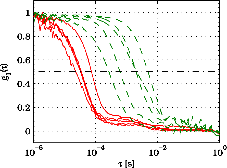

According to Sec. 2.3, the acquired measurements have been investigated both in terms of characteristic decay times ${\tau }_{0.5}$ [see Eq. (2)] and percentage variations $\mathrm{\Delta }{\tau }_{0.5}$ [see Eq. (4)] [no smooth function has been performed on the recoded $g_1(\tau )$ functions]. The obtained ${\tau }_{0.5}$ and $\mathrm{\Delta }{\tau }_{0.5}$ are shown in Figs. 7 and 8, respectively.

Fig. 7

Characteristic decay times ${\tau }_{0.5}$ relative to the five autocorrelation functions pairs acquired during the activities aimed at testing the ability to reveal ChBF variations (Fig. 6). For each pair, the ${\tau }_{0.5}$ recorded before the overpressure (${\mathrm{B}}^{(i)}$, $i\in [1,\dots ,5]$) is drawn with a circle (◯), whereas the ${\tau }_{0.5}$ recorded during the overpressure (${\mathrm{D}}^{(i)}$, $i\in [1,\dots ,5]$) is drawn with a square (□).

Fig. 8

Percentage variation $\mathrm{\Delta }{\tau }_{0.5}$ relative to the five autocorrelation functions pairs acquired during the activities aimed at testing the ability to reveal ChBF variations (Fig. 6). For each pair, the $\mathrm{\Delta }{\tau }_{0.5}$ recorded before the overpressure (${\mathrm{B}}^{(i)}$, $i\in [1,\dots ,5]$) is drawn with a circle (◯), whereas the $\mathrm{\Delta }{\tau }_{0.5}$ recorded during the overpressure (${\mathrm{D}}^{(i)}$, $i\in [1,\dots ,5]$) is drawn with a square (□).

3.3.

Moderate Temperature Increase

The second activity investigates the temperature rise consequent to TTT laser treatment.

The treatment settings are reported in Table 1.

At the end of the treatment, the ophthalmologist reported inappreciable visible alterations of the ocular fundus tissues.

Figure 9 shows the obtained autocorrelation functions. According to Sec. 2.3, the acquired measurements have been investigated both in terms of characteristic decay times ${\tau }_{0.5}$ [see Eq. (2)] and percentage variations $\mathrm{\Delta }{\tau }_{0.5}$ [see Eq. (4)] [no smooth function has been performed on the recoded $g_1(\tau )$ functions]. The obtained ${\tau }_{0.5}$ and $\mathrm{\Delta }{\tau }_{0.5}$ are shown in Figs. 10 and 11, respectively.

Fig. 9

Autocorrelation functions acquired during the activities aimed at testing the ability to reveal fundus temperature variations. The measurement acquired before the TTT treatment is drawn in continuous line (—), the measurements acquired during the treatment are drawn in dashed line (– – –) and, the measurements acquired after the TTT are drawn in bold continuous line (—). The horizontal dashed-dot line (– . – . –) indicates the $g_1(\tau )=0.5$ condition of Eq. (2).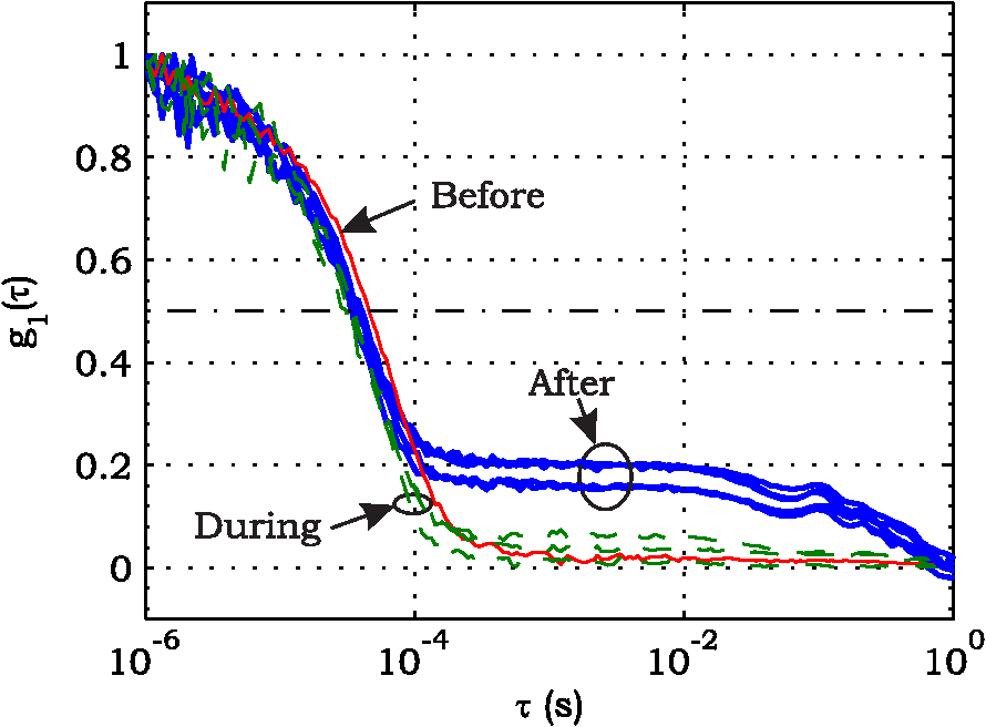

Fig. 10

Characteristic decay times ${\tau }_{0.5}$ relative to the autocorrelation functions acquired during the activities aimed at testing the ability to reveal fundus temperature variations (Fig. 9). The ${\tau }_{0.5}$ recorded before the laser treatment (${\mathrm{B}}^{(1)}$) is drawn with a circle (◯), the ${\tau }_{0.5}$ recorded during the treatment (${\mathrm{D}}^{(1)}÷{\mathrm{D}}^{(3)}$) are drawn with squares (□), and the ${\tau }_{0.5}$ recorded after the treatment (${\mathrm{A}}^{(1)}÷{\mathrm{A}}^{(5)}$) are drawn with diamonds (⋄). The wide rectangle in the background (pink in color version) indicates the TTT treatment.

Fig. 11

Percentage variation $\mathrm{\Delta }{\tau }_{0.5}$ relative to the autocorrelation functions acquired during the activities aimed at testing the ability to reveal fundus temperature variations (Fig. 9). The baseline $\mathrm{\Delta }{\tau }_{0.5}$ recorded before the laser treatment (${\mathrm{B}}^{(1)}$) is drawn with a circle (◯), the $\mathrm{\Delta }{\tau }_{0.5}$ recorded during the treatment (${\mathrm{D}}^{(1)}÷{\mathrm{D}}^{(3)}$) are drawn with squares (□), and the $\mathrm{\Delta }{\tau }_{0.5}$ recorded after the treatment (${\mathrm{A}}^{(1)}÷{\mathrm{A}}^{(5)}$) are drawn with diamonds (⋄). The wide rectangle in the background (pink in color version) indicates the TTT treatment.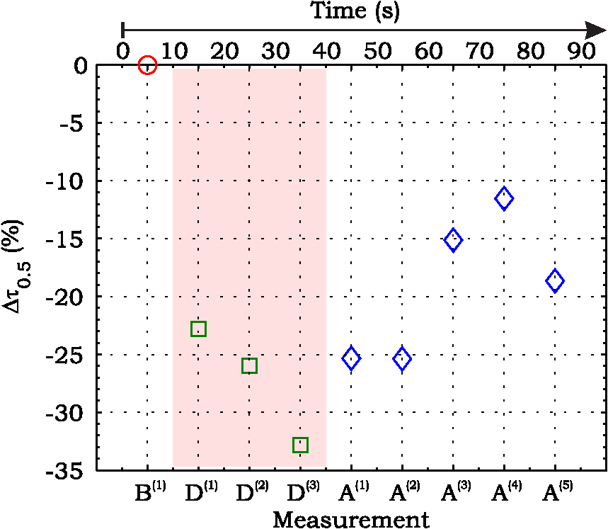

3.4.

Injection of Au-Nanoparticles

Finally, the ability to detect nano- and micro-aggregates carried by the ocular blood flow has been tested by injecting a bolus of Au-NPs in the ear vein of a rabbit. Data about the injected Au-NPs bolus are reported in Table 2.

Figure 12 shows the obtained autocorrelation functions. According to Sec. 2.3, the acquired measurements have been investigated both in terms of characteristic decay times ${\tau }_{0.5}$ [see Eq. (2)] and percentage variations $\mathrm{\Delta }{\tau }_{0.5}$ [see Eq. (4)] [no smooth function has been performed on the recoded $g_1(\tau )$ functions]. The obtained ${\tau }_{0.5}$ and $\mathrm{\Delta }{\tau }_{0.5}$ are shown in Figs. 13 and 14, respectively.

Fig. 12

Autocorrelation functions acquired during the activities aimed at testing the ability to detect nano- and micro-aggregate in ocular fundus circulation. The measurements acquired before the injection are drawn in continuous line (—), the measurements acquired during the injection are drawn in dashed line (– – –) and, the measurements acquired after the injection are drawn in bold continuous line (—). The horizontal dashed-dot line (– . – . –) indicates the $g_1(\tau )=0.5$ condition of Eq. (2).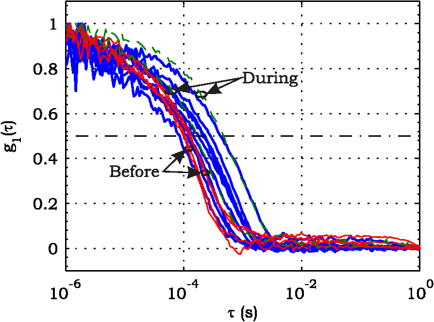

Fig. 13

Characteristic decay times ${\tau }_{0.5}$ relative to the autocorrelation functions acquired during the activities aimed at testing the ability to detect nano- and micro-aggregate in ocular fundus circulation (Fig. 12). The ${\tau }_{0.5}$ recorded before the nanoparticles (NPs) injection (${\mathrm{B}}^{(1)}÷{\mathrm{B}}^{(4)}$) are drawn with circles (◯), the ${\tau }_{0.5}$ recorded during the injection (${\mathrm{D}}^{(1)}÷{\mathrm{D}}^{(2)}$) are drawn with squares (□), and the ${\tau }_{0.5}$ recorded after the injection (${\mathrm{A}}^{(1)}÷{\mathrm{A}}^{(10)}$) are drawn with diamonds (⋄). The wide rectangle in the background (pink in color version) indicates the NPs injection.

Fig. 14

Percentage variation $\mathrm{\Delta }{\tau }_{0.5}$ relative to the autocorrelation functions acquired during the activities aimed at testing the ability to detect nano- and micro-aggregate in ocular fundus circulation (Fig. 12). The baseline $\mathrm{\Delta }{\tau }_{0.5}$ recorded before the NPs injection (${\mathrm{B}}^{(1)}÷{\mathrm{B}}^{(4)}$) are drawn with circles (◯), the $\mathrm{\Delta }{\tau }_{0.5}$ recorded during the injection (${\mathrm{D}}^{(1)}÷{\mathrm{D}}^{(2)}$) are drawn with squares (□), and the $\mathrm{\Delta }{\tau }_{0.5}$ recorded after the injection (${\mathrm{A}}^{(1)}÷{\mathrm{A}}^{(10)}$) are drawn with diamonds (⋄). The wide rectangle in the background (pink in color version) indicates the NPs injection.

4.1.

Discussion on the Measurement Uncertainty

As reported in Sec. 3.1, the recorded percentage experimental standard deviations of the sample ${\sigma }_{\%}$ were essentially less than 8%. Therefore, by introducing a sort of “safety factor,” the measurement uncertainty can be roughly estimated in about 10% (both for ${\tau }_{0.5}$ and $\mathrm{\Delta }{\tau }_{0.5}$ estimations, see Sec. 2.4).

Obviously, such 10% measurement uncertainty is not the measurement uncertainty relative to the analysis of blood flow, temperature variations or NPs, but the measurement uncertainty relative to ${\tau }_{0.5}$ and $\mathrm{\Delta }{\tau }_{0.5}$ estimations. As a result, the measurement uncertainty relative to the analysis of blood flow, temperature variations or NPs is reasonably higher than 10% and depends on the model used to joint such quantities—blood flow, temperature, and NPs—to the estimated ${\tau }_{0.5}$ or $\mathrm{\Delta }{\tau }_{0.5}$.

Actually, measurement uncertainty depends on both “intrinsic” factors such as the developed measurement procedure and measuring system and “extrinsic” factors relative to the environmental conditions, the investigated animal and the ophthalmologist that performs the measurements.

For instance, any relative motion between the measuring system and the measurand—the rabbit’s eye—results both in an apparent variation of $\langle \mathrm{\Delta }{r}^2(\tau )\rangle$ and a possible variation of the measuring site. Therefore, “extrinsic” factors such as movements of the investigated animal, i.e., due to different response to the sedatives and slight tremors of the ophthalmologist alter the measures, thus increasing the measurement uncertainty and possibly leading to measurement artefacts.

As an example, as previously stated $t_{\mathrm{meas}}>110÷120\mathrm{s}$ rapidly increases the measurement uncertainty. As shown in Fig. 2 the animal under test was immobilized by using a guillotine system and the GLC was hand-held by the ophthalmologist, thus such measurement uncertainty increase is reasonably an “extrinsic” factors depending on rabbit’s and/or ophthalmologist’s movements. Mechanical tools such as a stereotaxic head-holder can probably reduce rabbit’s movements; however, for human testing, such solutions are in general not suitable and a fixation target is usually the only mechanical tool exploited to prevent eye movements. Therefore, in order to reduce the effects of such extrinsic factor—relative motion between the measuring system and the measurand—we are now working on a mechanical system aimed at holding the GLC. Nevertheless, extrinsic factors can be reduced but obviously not eliminated.

From what has been said previously, the ultimate measurement uncertainty depends on both “intrinsic” factors such as the measurement procedure, the measuring system and the performed data analysis and “extrinsic” factors relative to the investigated measurand—animal model or patient—and/or the ophthalmologist. Therefore, the question whether the “ultimate” measurement uncertainty level of this system is sufficiently small to enable clinical applications is beyond the scope of this article.

4.2.

Discussion on the Analysis of the Variation of the Choroidal Blood Flow

The relation between IOP and ChBF has been investigated for a long time. Although preliminary animal experiments reported linear relationship, thus neglecting autoregulation, some autoregulation has been now demonstrated both in animal experiments^46–49 and human testing.^50–52

The ChBF regulation is known to be complex and to vary from subject to subject⁵² and the performed “handmade” pressure manipulation did not allow estimation of the induced IOP variation, thus it is difficult to estimate the induced blood flow variation. Nevertheless, in accordance with the expected ChBF reduction,^46–52 the observed $\mathrm{\Delta }{\tau }_{0.5}$ (Fig. 8) are significantly higher than the estimated 10% measurement uncertainty, thus confirming that the developed measuring system is able to detect ChBF variations.

Blood flow reduction results in a reduction of the $\langle \mathrm{\Delta }{r}^2(\tau )\rangle$ relative to “dynamic” scatterers—scatterers carried by the blood flow—thus according to Eq. (1), it is expected to result in an increased “characteristic” decay time ${\tau }_{0.5}$. Figures 6 and 7 clearly show that DCS is able to detect this phenomenon originated by an increased IOP.

The large variations shown in Figs. 6 and 7 are not surprising. According to the study performed by Kiel and Heuven on New Zealand albino rabbits,⁴⁷ an increase of the IOP from 10 mmHg to 100 mmHg can reduce by a factor of 10 the ChBF and similar results have been obtained analyzing Long-Evan rats.⁵³ Actually, ChBF reduction is due to both blood volume and velocity reductions. However, according to a recent study performed by Zhi et al. on Brown Norway rats,⁵⁴ from 10 to 50 mmHg, choroidal blood volume does not change, and at 60, 70, 80, and 100 mmHg, the choroidal blood volume, respectively, reduces of about 6.5%, 15%, 30%, and 80% of baseline. Therefore, up to 70 mmHg, choroidal blood volume basically does not change, whereas ChBF can be reduced by about seven times.⁴⁷ Since the examined retinal sites were chosen far away from visible retinal vessels, it means that up to about 70 mmHg, the IOP increase substantially influenced the movements of “dynamic” scatterers only, whereas optical properties basically did not change. Hence, by modeling the ChBF as random flow—$\langle \mathrm{\Delta }{r}^2(\tau )\rangle =\langle V^2\rangle {\tau }^2$—and roughly supposing a linear relationship between ChBF and square root of the mean square velocity $\langle V^2\rangle$—ChBF $\propto \langle V^2{\rangle }^{1/2}$—if ChBF reduces by a factor of $4÷7$ (i.e., approximately $40÷70\mathrm{mmHg}$), then $\langle \mathrm{\Delta }{r}^2(\tau )\rangle$ reduces by a factor of about $16÷49$. Such decorrelation statistically occurs at each scattering event with dynamic scatterers, thus leading to high responsivity.

Differences between the results (${\tau }_{0.5}$ and $\mathrm{\Delta }{\tau }_{0.5}$) obtained under different overpressure conditions are reasonably due to the poor repeatability of the performed handmade overpressures. Moreover, measurements may have been collected from slightly different fundus sites, thus also differences among the investigated regions may be responsible of the differences between the obtained decay times.

4.3.

Discussion on the Analysis of the Variations of the Fundus Temperature

According to Ibarra et al.,⁴⁵ the performed 200 mW TTT treatment (see Table 1) is expected to produce a fundus temperature rise lower than 2°C, whereas the threshold power settings for visible lesions in albino rabbits is about 950 mW (810 nm laser diode, spot-size 0.8 mm and, treatment duration 60 s), corresponding to retinal temperature increases of about 12°C.⁴⁵

Change in optical properties of the tissue—whitening—due to photocoagulation, corresponds to a denaturation of tissue proteins that occurs at approximately 18°C above basal temperature (i.e., 55°C). Nevertheless, protein denaturation is known to start under the photocoagulation threshold with a change in the folding of proteins starting at about $6÷12°\mathrm{C}$ above basal temperature.⁵⁵ Despite the gentle laser treatment, the developed measuring system has been shown able to detect the consequent moderate temperature increase. The $\mathrm{\Delta }{\tau }_{0.5}$ variations recorded as a function of the applied stimulus have been about three times higher than the estimated measurement uncertainty. Actually, temperature rising means increased thermal agitation, hence increased $\langle \mathrm{\Delta }{r}^2(\tau )\rangle$ of “semi-static” scatterers. According to Eq. (1), an increased $\langle \mathrm{\Delta }{r}^2(\tau )\rangle$ is expected to result in a ${\tau }_{0.5}$ reduction. Indeed, Figs. 9 and 10 show a ${\tau }_{0.5}$ reduction as a consequence of the gentle TTT treatment. The incomplete baseline recovery could be due to the temporary and/or permanently changes in protein conformations during TTT reported by Mainster and Reichel⁵⁶ and/or layered structure developing with a static layer. The analysis of such phenomena can be probably easily performed by using the two-cells model reported in our previous articles.^4–6

Actually, the ${\tau }_{0.5}$ reduction agrees with both an increased thermal motion and a physiologically increased blood flow aimed at dissipating the excess heat due to the TTT treatment. As reported in Sec. 2.4, the explored retinal region was chosen far away from visible vessels. Nevertheless, temperature-induced vasodynamics of choroids is known to be complex mechanism.⁵⁷ Indeed, in 1991, a human study from Parver⁵⁸ reported that ChBF increases as a consequence of the fundus heating, whereas a more recent human study from Nagaoka and Yoshida⁵⁹ in 2004 reported that ChBF decreases upon heating of the eye. Supposing that ChBF decreases upon heating of the eye, the observed ${\tau }_{0.5}$ reduction is therefore reasonably due to an increased thermal motion.

Actually, the small ChBF reduction reported by Nagaoka and Yoshida⁵⁹ was due to both reduced RBC velocity and reduced blood volume almost in equal measure. According to Eq. (1), reduced RBC velocity is expected to results in a $\langle \mathrm{\Delta }{r}^2(\tau )\rangle$ reduction, hence increasing ${\tau }_{0.5}$. On the contrary, reduced blood volume is expected to result in a reduction in the absorption coefficient, hence resulting in an increased mean path length $s$ and thus leading to a reduced ${\tau }_{0.5}$ (see Sec. 4.4). Therefore, such thermally induced ChBF reduction is expected to give rise to two phenomena that roughly compensate each other. As a result, the ${\tau }_{0.5}$ and $\mathrm{\Delta }{\tau }_{0.5}$ reductions shown in Figs. 10 and 11 reasonably confirm the ability to detect variations of the fundus temperature.

4.4.

Discussion on the Detection of Nano- and Micro-aggregates

Nano- and micro-aggregates carried by the blood flow are expected to change the fundus optical properties (${\mu }_a$ and ${\mu }_s$), thus potentially changing $P(s)$, $\langle q^2\rangle$ and, $l_s$. On the contrary, being the aggregates carried by the blood flow, no change is expected with respect to the $\langle \mathrm{\Delta }{r}^2(\tau )\rangle$ relative to the blood flow itself (“dynamic” scatterers).

As shown in Figs. 12 and 13, DCS is able to detect the Au-NPs transit and the subsequent physiological recovery. The obtained results are in accordance with the Au-NPs optical properties reported in a theoretical study by Jain et al.⁶⁰ According to Jain et al.,⁶⁰ the injected Au-NPs have ${\mu }_s/{\mu }_a\ll 1$, therefore the probability that photons have to be scattered by Au-NPs is extremely low. Moreover, Au-NPs have higher absorption compared to RBCs.⁶⁰ Hence, also considering the small injected volume (Table 2), Au-NPs injection roughly affects $P(s)$ only. Since the absorption coefficient ${\mu }_a$ describes the mean distance $l_a=1/{\mu }_a$ traveled by a photon before it is statistically absorbed, the higher the absorption coefficient and the lower the probability of long-path photons to be detected. Therefore, roughly supposing $\langle q^2\rangle$, $l_s$ and $\langle \mathrm{\Delta }{r}^2(\tau )\rangle$ to be the same all over the volume under test, from Eq. (1) it is easy to notice that a reduction in the path length $s$ results in a reduction of the $s/l_s$ ratio, hence resulting in an increase of the characteristic decay time ${\tau }_{0.5}$.

In agreement with the theoretical expectations, Figs. 12 and 13 show an abrupt increase in the ${\tau }_{0.5}$ as a consequence of the NPs injection. Then, the ${\tau }_{0.5}$ gradually returns to baseline during the physiological recovery.

Actually, both the effects due to: (a) the saline solution optical properties and, (b) the potential transient changes in blood pressure during the injection may have contributed to the ${\tau }_{0.5}$ variations. However, physiological saline solution has optical properties similar to pure water,⁶¹ thus negligible absorption compared to blood. As a result, physiological saline solution is expected to result in a (tiny) ${\mu }_a$ reduction, thus to result in a (tiny) increase in the path length $s$ hence, to result in a (tiny) reduction of the characteristic decay time ${\tau }_{0.5}$.

On the other side, accordingly to the discussion and the references reported in Sec. 4.2, i.e., Kiel et al.,^46–49 there is clearer evidence of autoregulation in the rabbit’s choroid. The performed NPs injection had a mean flow of about $0.02\mathrm{ml}/\mathrm{s}$ (see Table 2), thus it is reasonable to suppose it to lead to limited changes in blood pressure, hence leading to little or no effect on ChBF and volume. Moreover, it is reasonable to suppose the recovery time due to changes in blood pressure to be faster than the $\approx 45\mathrm{s}$ shown in Figs. 13 and 14.⁴⁶ Therefore, the results shown in Figs. 12–14 are reasonably due to nano- and micro-aggregates, thus confirming the ability to detect nano- and micro-aggregates.

4.5.

Discussion on the Data Analysis

The question of which data analysis method is more appropriate for a specific task is quite difficult to address.

As previously discussed, the proposed simplified data analysis method is not intended to replace the previous specialized data analysis methods^4–6 and new different data analysis methods may provide better performances and/or even simpler analysis. Actually, specific theoretical models allow obtaining more information and may be necessary for some particular applications. Nevertheless, to fully access the information offered by the data analysis methods so far proposed in the literature,^4,6 additional data such as ${\mu }_a$, ${\mu }_s$ and, the $\alpha$ and $\beta$ probabilities⁴ are required.

Regardless of the specific clinical situation, the more suitable data analysis method is probably the simpler one able to provide a measurement uncertainty lower or equal to the target measurement uncertainty—measurement uncertainty specified as an upper limit and decided on the basis of the intended use of measurement results.⁶² Unfortunately, as discussed in Sec. 4.1, measurement uncertainty depends on both “intrinsic” and “extrinsic” factors, thus resulting in extremely difficult to estimate. Nevertheless, the combined standard measurement uncertainty is reasonably greater than the individual standard measurement uncertainties associated with the input quantities in the measurement model,⁶³ thus some comparisons can be made based on the data available for the analysis—the input quantities.

The simplified analytical distribution form (SADF) proposed in our first article,⁴ supposes single-path in order to model the complicated photon path distribution in ocular fundus. In order to do so, it is necessary to know the thickness and the optical properties of the investigated ocular fundus layers. The higher the uncertainties in thickness and/or optical properties, the higher the uncertainty relative to the single-path SADF model. Therefore, the single-path SADF data analysis method can be useful when the thickness and the optical properties are known, whereas resulting less applicable when such quantities are less known. As an example, the coefficients used in the previous SADF⁴ were relative to pigmented rabbits ocular fundus, thus such model can not be directly applied for the analysis of albino rabbits.

The second data analysis method⁶ performs the inversion of the Laplace equation by using the CONTIN software, hence reasonably allowing to highly reduce the issues relative to the uncertainties in thickness and/or optical properties. However, CONTIN software is time-consuming, thus resulting less appealing for real-time analysis. Moreover, the severe nonorthogonality of exponentials leads to an ill-conditioned problem, hence the inversion of the Laplace integral suffers from the following problems:⁶⁴ (a) distortion in the $g_2(\tau )$ function due to nonideal experimental conditions such as baseline errors and nonuniform laser beam profile, (b) noise that do not exhibit the nature of exponential decay, and (c) limited delay-times range of correlators. As a result, the data analysis method based on the inversion of the Laplace integral requires accurate system design in order to avoid distortion in the $g_2(\tau )$ function and practically results less appealing for real-time analysis or the analysis of noisy datasets.

The proposed simplified data analysis methods—Eqs. (2) and (4), ${\tau }_{0.5}$ and $\mathrm{\Delta }{\tau }_{0.5}$—offer extremely easy interpretation of the experimental data and allow fluent implementation of real-time analysis. As an example, this is a clear advantage for all applications aimed at the definition of an end-point. Moreover, they neither relay on the knowledge of anatomical data nor perform the inversion of the Laplace integral, hence realistically resulting less sensitive to both (a) uncertainties in the thickness and the optical properties of the investigated ocular fundus and (b) nonideal experimental conditions and noises.

Actually, according to the reported results the ${\tau }_{0.5}$ analysis seems to be more sensitive to inter- and intra-individual variability than the $\mathrm{\Delta }{\tau }_{0.5}$ analysis. As a matter of fact, the ${\tau }_{\text{BASE}}$ values reported in Figs. 4, 7, 10, and 13 range from $\approx 20$ to $\approx 100\mu \mathrm{s}$. On the contrary, the $\mathrm{\Delta }{\tau }_{0.5}$ analysis seems to be robust to inter- and intra-individual variability. Indeed, the $\mathrm{\Delta }{\tau }_{0.5}$ variations recorded as a function of the applied stimulus have been always greater than the measurement uncertainty, thus potentially allowing to quantify the magnitude of each fundus variation—ChBF, temperature and nano- and micro-particles.

4.6.

Comparison with Other Measurement Techniques

As previously stated, DCS and Laser Doppler systems are based on the same physical principle and offer the advantage to provide noninvasive measurements of blood flow. However, Laser Doppler systems are based on confocal configurations, thus the volume probed by the detected photons is accordingly small. Moreover, single photon counting approach of DCS offers better performance in terms of sensitivity, hence allowing to better investigate the feeble signal arising from multiple-scattering.

Among ancillary tests in ophthalmic practice, OCT is probably the most commonly used. The OCT is a noncontact and noninvasive imaging technique widely used for human eye imaging.⁶⁵ The use of OCT in ophthalmology is not limited to a “static” analysis. As an example, when OCT is combined with Doppler analysis, it can be used to measure retinal blood flow,⁶⁶ and optical microangiography (OMAG) is capable of generating 3D dynamic perfusion images of tissue microcirculation.⁶⁷ Joint spectral and time domain optical coherence tomography (joint STdOCT) has been shown capable of three-dimensional quantitative imaging of retinal and ChBF,⁶⁸ and D-OMAG used in conjunction with and ultrahigh sensitive OMAG (UHS-OMAG) allows to obtain simultaneous 3D angiography and quantitative retinal blood flow measurement.⁶⁹

Moreover, OCT can be used to access TTT treatments outcome, i.e., as in Refs. 70 and 71. However, there is a latency in tissue denaturation after the laser is stopped⁵⁵ and this is probably one of the reasons why, to the best of our knowledge, there were no study reports about the use of OCT for determining an endpoint for TTT treatments.

On the contrary, the use of OCT for monitoring of NPs in biological tissues has been reported.^72,73

However, OCT systems are extremely complex systems based on a low coherence interferometer. As an example, in Time domain OCT the sample is scanned by changing the pathlength in the reference arm and the position of the measurement beam on the sample, respectively. Therefore: (a) the pathlength in the reference arm has to be scanned rapidly and precisely, (b) the amplitude of such pathlength variation must be large enough to cover the desired axial imaging range—the depth of volume under test—and (c) the position of the measurement beam has to be moved rapidly and precisely all over the volume under test ensuring appropriate focus, thus requiring complex scanning mechanisms. Then, the OCT image is composed by analyzing all the signals recorded for each reference arm pathlength and measurement arm position. Frequency domain OCT allows to avoid to change the pathlength in the reference arm, but it requires the use of a spectrometer for the analysis of the collected signal. Therefore, OCT systems require expensive optical and electronic components and complex software, hence resulting expensive systems.

On the contrary, in DCS systems, there are neither reference arms nor the scanning mechanisms and the dimension and the depth of the volume under test is simply determined by the distance between the illumination spot and the collection point. As a result, the integration of DCS system with OMs is easy and less expensive. As a matter of fact, the proposed DCS system has been integrated by simply using a beam splitter (Sec. 2.2) and the DCS system cost—excluding the OM—is about 10,000 dollars.

4.7.

Conclusions

From the discussion above, it is clear that the definition of the achievable metrological performances, i.e., responsivity and limit of detection, depends on several “intrinsic” and “extrinsic” factors. Therefore, there are currently no guarantees that the developed measuring system can definitely contribute in understanding and/or improving the current clinical issues and much more work will be needed before the proposed measuring system will reach clinical maturity. However, the reported results suggest that important diagnostic information can be obtained from DCS measurements of the ocular fundus.

The ability to detect ChBF variations can be useful both in fundamental research and practical clinical applications. Indeed, even though the ability to detect ChBF variations has been tested by increasing IOP, the system capability to reveal ChBF variations is reasonably not limited to the analysis of perturbations induced by pressure variations.

The ability to detect variations in the fundus temperature can be useful in managing TTT, PDT, and DEP, thus allowing to avoid or reduce treatment complications.

The ability to detect nano- and micro-aggregate could allow both diagnoses when the presence of such aggregates is related to specific diseases, i.e., diseases related to the environmental pollution and verifying for instance the impact of NPs injection in nanomedicine. Moreover, the state of aggregation of the NPs affects their optical properties, hence in general affecting $P(s)$, $\langle q^2\rangle$, and $l_s$. As a result, DCS also theoretically allows investigation of variations in the state of aggregation of the flowing NPs. However, the proposed data analysis do not allow to differentiate between $g_1(\tau )$ variations due to variations in NPs concentration or state of aggregation. As a result, the NPs state of aggregation can be investigated only if the NPs concentration inside the sample is known or it does not change among the various measurements.

Finally, Au-NPs are not only a suitable test to investigate the ability to detect nano- and micro-aggregates in blood circulation, but also a good option for DPE. According to Jain et al.,⁶⁰ the Au-NPs shape and dimension can be tailored in order to obtain the desired absorption and scattering spectra, thus resulting in a suitable dye for DEP. Nevertheless, DCS is theoretically able to detect any dye that affects any of $P(s)$, $\langle q^2\rangle$, and $l_s$. Therefore, no restriction is theoretically imposed on dye selection for DEP.