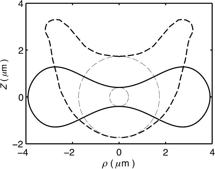
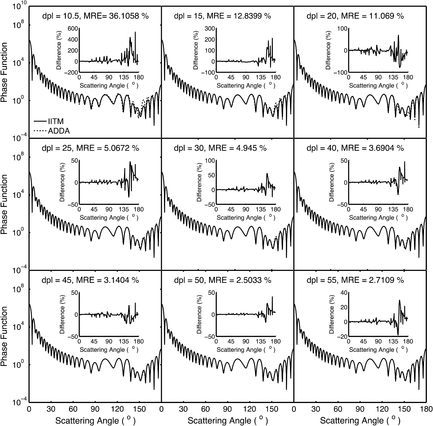
1.

Introduction

Red blood cells (RBCs) or erythrocytes flowing in blood are responsible for the delivery of oxygen from the lungs throughout the human body and the return transport of ${\mathrm{CO}}_2$ from the tissues to the lungs. RBCs have specific biophysical properties for responding to a change in the local chemical and mechanical environment. The deviations from regular biophysical properties of RBCs impair their normal functions in the human body and are sensitive markers for various blood disorders and diseases, e.g., malaria and sickle cell anemia. For this reason, relevant techniques to obtain the characteristics of the biophysical properties of RBCs have been of paramount significance in medical diagnostics. Optical techniques have been considerably investigated as they provide a fast and noninvasive pathway to probe cell changes. Some of the well-known examples of optical techniques are flow cytometers,^1,2 quantitative phase imaging,^3,4 and Fourier transform light scattering.⁵

To interpret optical experimental data and extract accurate and significant RBC information, computational techniques are required to model single-scattering properties of RBCs. Normal mature RBCs are shaped as biconcave oblate discs, which deform with pressure and physiological conditions in blood. The disc diameter ranges from 5 to 10 μm. Microcyte and macrocyte⁶ are, respectively used to identify RBCs with diameters smaller than 7.0 μm and larger than 8.5 μm. Although the RBC shape is intriguing, performing rigorous light scattering calculations is a nontrivial task; particularly prior to the twenty-first century. In most of the earlier optical modeling, theoretical simplifications had to be made. Examples of such simplifications include the spherical^2,7 and spheroidal⁸ approximations of the RBCs’ morphology made because of the ease with which the optical properties can be obtained from either the Lorenz-Mie theory or the extended boundary condition method (EBCM). Other examples of the simplifications are the use of approximate or semi-empirical scattering computational methods to compute the optical properties of more realistic RBC shapes, such as the Born approximation,⁹ anomalous diffraction theory,^10,11 Wentzel-Kramers-Brillouin approximation,¹² and physical-geometric-optics approximation method.¹³ As the numerical methods have gradually developed to solve Maxwell’s equations, numerous publications are available on light scattering by RBCs using numerically rigorous methods including the discrete-dipole approximation (DDA),^14,15 finite-difference time-domain (FDTD) method,¹⁶ boundary element method,¹⁷ multilevel fast multipole algorithm (MLFMA),¹⁸ and discrete sources method (DSM).^19,20 To model light scattering signals associated with deformed RBCs²¹ in Poiseuille flows, the FDTD method has been employed. Moreover, the MLFMA has been applied to distinguish light-scattering signals from healthy and diseased RBCs.¹⁸

Among the available computational methods, two T-matrix methods, EBCM and DSM, are expected to be the most appealing because they are semi-analytical (i.e., low demand on computer memory and high accuracy of derived results) and efficient in obtaining the optical properties of a particle with multiple possible orientations. The motivation for applying the T-matrix methods to obtain the optical properties of RBCs is additionally justified by the axial symmetry of most RBCs. However, the standard EBCM to compute the T-matrix encounters the ill-condition problem, because RBCs are concave and fairly flat. As to the other T-matrix methods, both the DSM and null-field method with discrete sources have been applied to the optical modeling of RBCs. A comparison between the DSM and the DDA methods shows large differences²² that are attributed to the failure of the DSM to converge. The numerical methods, the DDA and FDTD, have been much more popular than the other available T-matrix methods in practical modeling, although computationally intensive when the particle size parameter is large.

Two recent papers^23,24 report on the results of light scattering by excessively large spheroidal and cylindrical particles based on the invariant imbedding T-matrix method (II-TM) that combines the method of separation of variables (SOV) or EBCM and an invariant imbedding method (IIM)²⁵ to compute the T-matrix (the two methods are referred to as $\mathrm{SOV}+\mathrm{IIM}$ and $\mathrm{EBCM}+\mathrm{IIM}$). Either the $\mathrm{SOV}+\mathrm{IIM}$ or $\mathrm{EBCM}+\mathrm{IIM}$ is demonstrated to be applicable to particles of an aspect ratio much larger than the values that can be effectively handled by the EBCM. The role of the SOV and EBCM is to enhance the numerical performance of the IIM. Because of the significance of RBCs’ light scattering in a biological system, the purpose of this study is to illustrate the numerical capability of the II-TM in the optical modeling of RBCs. This research will not extensively compare the II-TM with other available methods; instead, it will contrast the II-TM with the DDA. A better understanding of the relative numerical performance of the II-TM in comparison with the other methods can be gained by comparing the DDA method with other numerical methods reported in Wriedt et al.²⁶ and Gilev et al.²²

The remainder of this work is organized into five sections. Section 2 describes the morphology of RBCs, followed by the discussion of complex refractive indices in Sec. 3. Section 4 contains the procedures necessary to apply the II-TM to solve the light scattering by RBCs. The numerical simulation results are presented and discussed in Sec. 5. A summary of the present study and a conclusion of the optical modeling applicability of the II-TM are delineated in Sec. 6.

2.

Morphology of RBCs

A normal RBC is generally shaped as a biconcave disk to achieve a large surface-area-to-volume ratio. Figure 1(a) shows the typical model geometry of RBCs considered to be axially symmetric. The meridional cross-section of a biconcave RBC is shown in Fig. 1(b) with four characteristic morphological parameters,²⁷ i.e., the diameter ($D$), dimple thickness ($t$), maximum thickness ($h$), and diameter of a circle that determines the location of the maximum thickness ($d$).

Fig. 1

(a) 3-D RBC model; (b) two-dimensional cross-section; and (c) five different parametric models.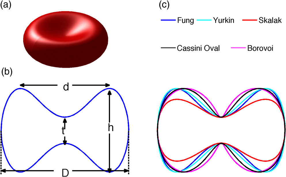

The diameter measurements of RBCs can be traced back to 1821 (see Table 2 in Ponder²⁸). In 1971, Evans and Fung²⁹ significantly improved the resolution of RBC geometric measurements by using the interference holography technique and, based on the analysis of 50 cells, reported an average diameter of 7.82 μm, a dimple thickness of 0.81 μm, and a height of 2.58 μm. Ten years later, using the same technique but a much larger sample, 1581 cells from 14 healthy people, Fung et al.³⁰ reported an average diameter of 7.65 μm, a dimple thickness of 1.44 μm, and a height of 2.84 μm. The parameters of an averaged RBC from the two measurements are used in the optical modeling found in Sec. 5. The values of RBC parameters reported in the literature and obtained from different techniques can be found in Fung et al.³⁰ and Yurkin.²⁷ The volume ($V$), the surface area ($S$), and the sphericity index ($\mathrm{SI}=4.836V^{2/3}/S$) are important geometric parameters. In the hematocrit study, a three-parametric mathematical model is proposed to characterize the geometry, from which $V$, $S$, and $\mathrm{SI}$ can easily be computed after the minimization of the difference between the model and the data image.

The parametric equation of the Evans-Fung model is given by²⁹

In the Evans-Fung and Yurkin models, the parametric coefficients are completely determined once $D$, $t$, $h$, and $d$ are known and vice versa. However, it should be mentioned that the parametric equations given by Eqs. (2) and (3) could not be of the expected biconcave shape. To illustrate this feature, the values of $D$, $t$, and $h$ are fixed at the averaged values reported in Evans and Fung with the parameter $(\zeta =d/D)$ varying in the range between 0.05 and 0.95. We found that the shape given by Eq. (1) is not a biconcave shape when $d/D$ is smaller than approximately 0.6 (i.e., $d=4.692$) or larger than 0.89 (i.e., $d=6.9598$), as evident in the three top panels of Fig. 2, which show typical geometries determined in Eq. (1). The results indicate that the parametric model based on Eq. (1) has a limited range of the parameter $d$. Because $d$ is rarely reported in experiments, $c_0$, $c_1$, and $c_2$ cannot be determined only based on $D$, $t$, and $h$. The extra morphological parameters can be specified through the determination of the particle volume, the particle surface area, or other geometric parameters. Similarly, we plotted the three typical geometries shown in the lower panels of Fig. 2 according to the Yurkin model. When $\zeta$ is smaller than $\sim 0.31$, the resultant geometry is not the expected shape, and the dimple thickness is larger than the given value. The reason for failing to obtain the expected geometry is due to the existence of different branches of geometry. Figure 3 shows the variation of the particle volume, the surface area, and $\mathrm{SI}$ as a function of $\zeta$. The Yurkin model has a larger range of deformation. The volume and $\mathrm{SI}$ index predicted from the Yurkin model are always larger than those of the Evans-Fung model. The surface area of the Yurkin model is smaller than that of the Evans-Fung model when $\zeta$ is less than 0.87.

Fig. 2

The shape of RBCs determined by Eq. (1) (upper panel) and Eq. (3) (lower panel) for three different values of $\zeta$.

Fig. 3

Volume, surface area, and sphericity index of the Evans-Fung and the Yukin models as a function of $\zeta$.

The geometry of RBCs depends on many factors associated with the pressure and physiologic conditions in blood. Skalak and Branemark³³ discovered that an RBC deforms into a parachute shape in order to traverse capillaries smaller than the diameter of the nondeformed RBC. Zarda et al.³⁴ developed a finite element method to model the deformation of RBCs from a biomechanics approach. Based on the lubrication theory, Secomb³⁵ studied RBC deformation for both axisymmetric and fully 3D geometries. Pozrikidis³⁶ employed a boundary-integral method to model axisymmetric motion of RBCs passing through capillaries. Hosseini and Feng³⁷ studied the deformation of RBCs using a particle-based model. To illustrate the numerical capability of the II-TM to model deformed RBCs, we use the geometry reported by Zarda et al.³⁴ corresponding with a dimensionless pressure drop of 16. The results are shown in Fig. 4.

Fig. 4

Deformed RBC due to pressure drop in poiseuille flow. The inscribed sphere of a deformed RBC is larger than that of a normal RBC.

3.

Complex Refractive Index

In addition to the size and morphology of a RBC, the complex refractive index is required to theoretically determine the optical properties. RBCs consist of a membrane filled with hemoglobin solution. The membrane is thin, on the order of 7 nm, and its influence on scattering was usually neglected, but the appropriateness of neglecting the membrane in scattering computation was confirmed through numerical calculations based on the finite element method.¹⁷ For this reason, RBCs are considered to be homogenous, and the major determination for the refractive index is the hemoglobin concentration.

The RBCs’ refractive indices at various wavelengths have been reported in the literature. Prahl³⁸ tabulated the molar extinction coefficient for both oxygenated and deoxygenated hemoglobin in water, and the imaginary part of the refractive index can be obtained from the result. Friebel and Meinke^39,40 measured the absorption coefficient of hemoglobin as well as the reflectance from which the complex refractive indices are derived. The comparison of the absorption coefficient compiled by Prahl,³⁸ and the measurement by Friebel and Meinke³⁹ finds the data are close, although some small differences can be identified. To obtain the real parts of refractive indices, Faber et al.⁴¹ applied the subtractive Kramers-Kronig relations to the absorption data tabulated by Prahl.³⁸ Zhernovaya⁴² reported the real parts of refractive indices for nine wavelengths between 400 and 700 nm for both oxygenated and deoxygenated hemoglobin. The real parts of the refractive indices reported from the previous studies are quite different. In this modeling, we follow Faber et al.⁴¹ because the complex refractive indices in the spectral range 250 to 1000 nm can be easily obtained, although the data may not be accurate due to the finite range of absorption spectrum. Figure 5 shows the variation of the complex refractive indices with respect to the wavelength.

Fig. 5

Complex refractive index of oxygenated and deoxygenated hemoglobin.

4.

Invariant Imbedding T-Matrix Method

The wavelength of the incident light of general interest is from the UV to the near infrared. In this wavelength range, the maximum size parameter of RBCs is on the order of 200. Although the optical properties may be derived from available numerical methods based on advanced parallel computational techniques, the computation is too intensive, particularly in the case of a large number of simulations associated with multiple orientations, wavelengths, and sizes. We briefly summarize the II-TM for the computation of the single-scattering properties of RBCs.

The electromagnetic fields in light-scattering systems satisfy the Maxwell equations and can be expanded in terms of vector spherical functions. The T-matrix is defined to transform the expansion coefficients of the incident field and those of the scattered field. The basic principle of the II-TM to compute the T-matrix of a single RBC is illustrated in Fig. 6. The RBC is discretized in terms of multiple inhomogeneous spherical layers. The key procedure of the II-TM is to obtain the T-matrix of a particle composed of $k+1$ layers based on the T-matrix of a particle of $k$ layers. The T-matrix of the inscribed sphere is obtained from the separation of variables method (i.e., the Lorenz-Mie theory). One advantage of the II-TM is the simplicity with which it modifies the particle geometry and refractive index. For the detailed mathematical procedures and physical interpretations to calculate the T-matrix, please refer to our previous publications.²³

Fig. 6

Schematic diagram illustrating the principle of the II-TM to calculate the T-matrix, which contains all the light scattering information.

To adapt the parametric model into the II-TM package, one must solve the intersection of a sphere with the biconcave curve. To be more specific, the cosine of the polar angle (the angle between the radius and the positive symmetric axis), $\mu$, is required. In the Evans-Fung model, we have

5.

Results and Discussion

5.1.

Comparison of the II-TM and the DDA

Several reasons exist for comparing the II-TM and the DDA in the computation of RBC optical properties. First, the DDA method is applicable to arbitrarily shaped particles, and its accuracy is well understood through comparison with the other existing numerical methods. Therefore, the comparison of the II-TM and the DDA helps to gain knowledge of the relative performances of available numerical methods, validate the numerical implementation of the II-TM, understand the accuracy of the DDA, and choose the method of preference in practical applications. Moreover, RBCs in plasma or other solutions are optically soft, and the DDA’s performance is relatively better than the other available numerical methods. We use the Amsterdam DDA (ADDA) code (adda-0.79) developed by Yurkin and Hoekstra^27,43 (the original source code can be obtained at http://code.google.com/p/a-dda/).

Figure 7 shows the comparison of phase functions computed from the II-TM and ADDA for a RBC in the case of face-on light incidence. The wavelength ($\lambda$) of the incident light is 0.6328 μm in vacuum and 0.4747 μm in medium. The morphological parameters for the RBC are specified as: $D=7.82\mu \mathrm{m}$, $h=2.58\mu \mathrm{m}$, $t=0.81\mu \mathrm{m}$, and $d=4.843895\mu \mathrm{m}$; the size parameter defined in terms of the wavelength in the medium is $\pi D/\lambda \cong 51.7532$; and the relative refractive index is assumed to be 1.05. Either the KF model or the Yurkin model with $R_4=1$ is used to characterize the RBC shape. Multiple ADDA simulations are performed by increasing the number of dipoles per incident wavelength (dpl) from 10.5 (default value) to 55. To quantify the difference between the ADDA and the II-TM results, the mean relative error (MRE) is defined as

Eq. (9)

$$\mathrm{MRE}=100\%\frac{1}{N}\sum _{i=1}^N[P_{\mathrm{ADDA}}({\theta }_i)-P_{\mathrm{II}-\mathrm{TM}}({\theta }_i)]/P_{\mathrm{II}-\mathrm{TM}}({\theta }_i),$$

where $N$ ($=721$) is the number of scattering angles involved in the computations. As shown in Fig. 7, the ADDA phase functions expectedly approach the T-matrix result (i.e., the decrease of MRE indicated in the figure) with an increase in the dpl. When the number of dpl is larger than 25, the phase functions computed from the two methods are virtually very close. If the number of dpl is larger than 50, a further increase in the dpl does not necessarily decrease the mean relative error. The default dpl (10.5) is sufficient for the convergence of the DDA-simulated phase function in the forward hemisphere, in agreement with the literature,^14,27 but larger dpl (25) is needed for the convergence in the near-backscattering directions.

Fig. 7

Comparison of phase functions computed from the II-TM and the ADDA.

Figure 8 shows the comparison of phase functions, the $P_{12}$ and $P_{22}$ elements, computed from the ADDA and the II-TM for three different orientations with respect to the incident light corresponding to ${\theta }_{\mathrm{inc}}=30\mathrm{deg}$, 60 deg, 90 deg. The scattering plane ($y–z$ plane) is chosen for the phase matrix presentation. For convenience, the other 13 elements in the scattering phase matrix are not plotted. In the ADDA computation, the number of dpl is assumed to be 50. A good agreement is obtained except the $P_{12}$ element in the first column has a relative large difference at the scattering angle near 135 deg.

Fig. 8

Comparison of the phase function ($P_{11}$), $P_{12}$, and $P_{22}$ at three incident angles computed from the II-TM and ADDA. The scattering plane is chosen to be the $y-z$ plane (90 deg of scattering azimuthal angle).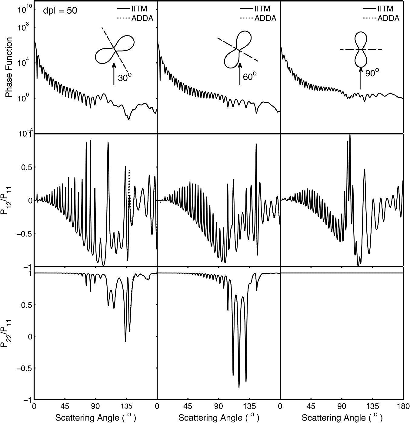

Figure 9 shows the comparison of six nonzero phase matrix elements for randomly oriented RBCs computed from the II-TM and the ADDA. To achieve the computational efficiency without losing significant accuracy, we have assumed the “dpl” to be 15 in the ADDA simulation. Note that the II-TM and the ADDA fundamentally differ in obtaining the orientation-averaged optical properties; the II-TM employs an analytical algorithm after the T-matrix is obtained while the ADDA computes the phase matrix for each orientation and then performs the numerical average. In the DDA simulations, as many as 64 numbers of $\alpha$ in (0, 360], 65 numbers of $\beta$ in (0, 90], and 1 number of $\gamma$ (0 is assumed) are set to achieve the randomness of RBC orientations; $\alpha$, $\beta$, and $\gamma$ are three Euler angles used to specify the orientation of the RBC in the laboratory coordinate system.

Fig. 9

Comparison of six nonzero phase matrix elements of randomly oriented RBCs computed from the II-TM and ADDA.

In order to compare the numerical performance (memory consumption and computational speed) of the II-TM and ADDA, Table 1 lists the computational time, the memory requirement, and the number of processors used in the computation. Note that for fixed orientations, the phase matrices are only computed referring to a specific scattering plane to hasten the ADDA. As seen from Table 1, both the II-TM and the ADDA are relatively efficient when the incident light is aligned with the RBC axis of symmetry. With this particular RBC orientation with respect to the incident light, a sub T-matrix rather than a whole T-matrix in the II-TM is required to compute the phase matrix, and the ADDA needs to run one simulation case associated with $X$ (or $Y$) polarization of the incident light. The evidence shows the ADDA is faster than the II-TM for a single orientation of the particle and much slower than the II-TM for randomly oriented RBCs. The reason is that most of computational time in the DDA simulations is spent on computing the scattered field because the internal field can be efficiently obtained for optically soft particles due to efficient convergence of the iterative solver. For example, the ratio of computational time for internal electric fields and phase matrix is approximately 0.87 in the case of the last row in Table 1. Differently, the T-matrix method is relatively efficient to obtain the phase matrix and spends a majority of time to calculate the T-matrix. In the three considered cases, the computational time of the phase matrix from the T-matrix is almost negligible. It should be pointed out that, in the II-TM simulations, we have employed a larger number of spherical layers with a step size of 0.05 and 100 terms of vector spherical harmonics in expanding the electric field to provide benchmarks. Numerical tests show that the two conditions can be relaxed without losing much accuracy, and the computational time can decrease. In the case of face-on incidence, for example, with the use of 0.1 step size and 82 terms of vector spherical harmonics, the computational time of II-TM is approximately two minutes with MRE of 2.189%. Also, note that the ADDA requires much more computer memory than the II-TM.

Table 1

Computational time, memory requirement, and number of processors involved in simulation.

$D$ (μm)	Orientation	II-TM			ADDA
		Time	Mem	Procs	Time	Dpl	Mem	Procs
7.82	0 deg	10.8 m	7 MB	1	3.8 m	15	3.6 G	1
					3.3 m	30	23 G	16
					5.2 m	50	110 G	64
	30 deg	11 m	0.2 G	16	8.9 m	15	3.6 G	1
					1 m	15	3.6 G	16
					11.3 m	50	110 G	64
	Random	11 m	0.4 G	16	6.77 h	15	3.6 G	16

5.2.

Oxygenated and Deoxygenated RBCs

After the validation of the II-TM method, we compute the optical properties of oxygenated and deoxygenated RBCs in a spectral range from 0.25 to 1.0 μm, an area in which the absorption of the medium can be reasonably neglected. In the spectral region beyond 1.0 μm, the absorption behavior of the medium becomes obvious. In this case, the theory of light scattering in an absorbing medium should be employed; therefore, we only consider wavelengths where the medium is nonabsorbing. In the computation, we assume that the plasma medium has the refractive indices of water.⁴⁴

Figure 10 shows the six phase matrix elements of an oxygenated and deoxygenated RBC at the Soret absorption band (415 nm). The particle is assumed to be randomly oriented. The phase function has relatively small differences; however, large differences are found for the $P_{22}$, $P_{33}$, and $P_{44}$ elements when the scattering angle is larger than 90 deg. The simulated results reveal that it may be possible to determine the degree of oxygen saturation based on the depolarization of backscattering light.

Fig. 10

Comparison of six nonzero phase matrix elements of randomly oriented oxygenated and deoxygenated RBCs at the Soret band.

Figure 11 shows the scattering and absorption cross-sections of oxygenated and deoxygenated RBCs in a spectral range from 0.25 to 1.0 μm. For comparison, we included the simulation results based on assuming the RBCs to be the volume-equivalent spheres. The dependence of the optical properties on oxygen saturation is evident. Despite the significant difference in geometry, the absorption cross-sections for biconcave RBCs and spherical RBCs are found to be close with the only observable differences near the Soret absorption band. However, the scattering cross-sections and, thus, the single-scattering albedo are more sensitive to the particle shape. In radiative transfer simulations, the nonsphericity of RBCs may need to be considered.

Fig. 11

Spectral variance of the scattering cross-section and absorption cross-section of oxygenated and deoxygenated RBCs.

5.3.

Deformed Red Blood Cells

The II-TM is adapted to compute the optical properties of deformed RBCs. Figure 12 illustrates the difference between the phase matrix of biconcave and parachute RBCs for face-on incidence. The incident wavelength is 660 nm, the refractive index of the medium is 1.331, and the relative refractive index of the RBC is $1.046+i1.261\times {10}^{-5}$. The RBC shape is modeled using the Evans-Fung parametric equation with $D=7.82\mu \mathrm{m}$, $h=2.58\mu \mathrm{m}$, $t=0.81\mu \mathrm{m}$, and $d=4.844\mu \mathrm{m}$. Because of the axial symmetry, we observe the phase function to oscillate and $P_{11}=P_{22}$ and $P_{33}=P_{44}$. The locations of peaks and minima are rarely the same because the phase delay of the incident light is quite different due to the thickness dissimilarity. Figure 13 mimics Fig. 12 except for the rim-on incidence. The phase matrix elements are averaged over the scattering azimuthal angle. We observe the near-backscattering phase function of biconcave RBCs is smaller than the parachute RBCs because the geometric cross-section of the former is smaller. $P_{22}/P_{11}$ is found to be quite unalike for the two different geometries. We have compared the ADDA results and the II-TM results for deformed RBCs and congruence is obtained when the dpl is 30. For simplicity, the ADDA results are not included.

Fig. 12

Comparison of phase matrix of biconcave and parachute RBCs. The incident light is aligned from below with the symmetry axis.

Fig. 13

Comparison of phase matrix of biconcave and parachute RBCs. The incident light makes an angle of 90 deg with the symmetry axis.

Figure 14 shows a comparison of the modified intensity corresponding to the scattering cases in Figs. 12 and 13. The modified intensity is defined as²⁷

Eq. (10)

$$P_{\mathrm{mod}}({\theta }_i)=P_{11}({\theta }_i){\sin }^2\left(\pi \frac{{\theta }_i-{\theta }_1}{{\theta }_n-{\theta }_1}\right),$$

where ${\theta }_i$ is the scattering angle, and ${\theta }_1$ and ${\theta }_n$ are chosen to be 10 and 50 deg. Equation (10) is used in the reverse light scattering for straightforward comparison of the simulated results with measurements by the scanning flow cytometer. The comparison of results shown in Fig. 14 illustrates distinguishable signals from biconcave RBCs and parachute RBCs.

Fig. 14

Modified intensity of the biconcave RBC and the parachute RBC for the face-on incidence (a) and the rim-on incidence (b).

5.4.

Statistical Average Properties

To compute the phase matrix of an ensemble of RBCs, we assume the sample to be diluted and the independent scattering assumption to be valid. In the modeling, we randomly generated RBCs according to the distribution given by Fung et al.³⁰ In Fig. 15, the histograms in terms of diameter, maximum thickness, minimum thickness, $d$, volume, and surface area are plotted. For simulation simplicity, we assume the RBCs to be randomly oriented. We compare the phase matrix computed from biconcave RBCs and spheres as shown in Fig. 16. The difference in the results predicted from spherical and biconcave models is found to be quite large. In addition to the nonsphericity indicator, $P_{22}/P_{11}$, the distinctive feature of the other phase matrix elements computed from a biconcave disk model is that the curves are smooth without oscillations. Collective scattering may be obvious when the sample is not diluted. In this case, further development is required for the present T-matrix method to consider mutual interactions between individual RBCs.

Fig. 15

Statistical distribution of RBC parameters.

Fig. 16

Comparison of statistical averaged phase matrix elements of randomly oriented RBCs and spheres.

6.

Summary and Conclusion

The II-TM has been applied to the simulation of optical properties of single RBCs. The II-TM is capable of obtaining the RBC optical characteristics in the wavelength spectrum from the UV to near-IR with realistic size parameters. Moreover, available parametric models reported in the literature to mimic the RBC shape have been implemented into the II-TM computational package developed by the authors.

When comparing the II-TM with the DDA method, a numerical method for the solution of light scattering by RBCs, excellent agreement between the two is obtained. The differences between the DDA results and the II-TM results decrease with an increase of the resolution in discretizing the RBC into discrete dipoles. The DDA method requires more computer memory than the II-TM because the former is a numerical method based on the dipole representation of the geometry and the latter is a semi-analytical method using spherical shells to discretize the particle geometry. However, when the number of particle orientations and the scattering angles is small, the DDA is comparable or even faster than the II-TM.

In summary, the II-TM can obtain accurate optical properties of RBCs in a wide range of size parameters with reasonable computational time. The extension of the present work to multiple red blood cells or other types of cells can be performed without much technical difficulty. The II-TM results can also be employed as a reference for the other numerical and approximate methods used by the research community.