1.

Introduction

Interventional guidance systems are becoming increasingly common in modern surgical procedures including open, laparoscopic, and robotic surgeries.¹ During such procedures, surgeons can lose track of tumors as they move in and out of the camera’s field of view. Guidance systems can be used to alleviate these concerns by providing a fusion of video with other imaging modalities, such as intraoperative ultrasound (US), to aid the surgeon in locating tumors or other regions of interest. The clinical utility of these guidance systems depends on the registration of other surgical tools and devices with the guidance system, such as stereoscopic endoscopes and US transducers.

The registration between US images and video visualization remains a significant challenge. Typically, electromagnetic (EM) or optical navigational trackers^2,3 are used to provide real-time position and orientation about tools such as US probes and endoscopic cameras. These navigational trackers, usually track sensors or markers, relative to a separate base station placed within the surgical setting, adding complexity. However, this approach has serious limitations and is subject to error buildup from multiple tracking and calibration errors.

EM-based surgical navigation and tracking systems^3,4 are the most common choice for laparoscopic surgery, flexible endoscopy, and other minimally invasive procedures because a clear line of sight is not required between the base station and the attached sensors (see Fig. 1). However, there are several drawbacks associated with using an EM-based system. First, wired EM sensors must be placed on the US transducer before it can be tracked by the surgical navigation system. This could decrease the surgeon’s comfort while potentially increasing the cost associated with handling and sterilizing modified surgical tools. Second, a large intrusive EM base station must be placed in close proximity with the operating table, adding clutter to the surgical setting. Third, EM-based systems also suffer from magnetic field distortions when metallic objects are placed within its field. This drawback is particularly significant as the tracked sensors will have significant errors when this is the case.

Fig. 1

(a) Standard electromagnetic-based navigation system and (b) photoacoustic (PA) navigation system.

Optical tracking systems such as those developed by Claron Technology Inc. (Toronto, Ontario, Canada) or Northern Digital Inc. (Waterloo, Ontario, Canada) avoid the field distortion problems associated with EM trackers and frequently do not require wired sensors. Studies have shown that optical trackers can detect their optical markers with submillimeter accuracy,^5,6 but line-of-sight restrictions often make them impractical for laparoscopic procedures. Markers can certainly be placed outside the body, but this will degrade the tracking accuracy for long and flexible tools inserted into the body.

Another drawback for both optical and EM-based systems is the need to acquire the transformation from the tool to the surgical navigation system indirectly, i.e., the transformation of interest is computed via a chain of transformations over several coordinate systems. This case applies to both EM and optical tracker-based systems. As an example, a transformation of interest would be one that goes from the EM base station’s coordinate system to the US image’s coordinate system. To acquire this transformation, one must obtain both the transformation from the EM base station to the EM marker and the transformation from the EM marker to the US image. The first transformation is given by the tracking information from the EM base station and the second must be obtained through a calibration process. Calibration is a topic where many authors have presented research to achieve better accuracy and lower errors.^7,8 Their results have shown that the calibration process dominates the overall error in the registration.^5–7 Other studies have presented overall registration errors of approximately 1.7 to 3 mm for artificial phantoms and 3 to 5 mm for tissue.^3,4,9,10

Yip et al.¹⁰ demonstrated a registration method that utilizes a tool at the air and tissue boundary. This tool had optical markers in the stereo camera (SC) space on one side and US-compatible fiducials on the other. A drawback of this method is that it requires a custom registration tool to be in direct contact with the tissue. Also, the US fiducials must be segmented from US B-mode images. This can be a difficult task as the speckle or structural information contained in US B-mode images may obscure the US fiducials.

Vyas et al.¹¹ demonstrated proof of concept for a direct registration method with the photoacoustic (PA) effect requiring a single transformation between the frames of interest as opposed to a chain of transformations. This method addresses each of the drawbacks above. Markers or sensors are not necessary to generate a coordinate transformation between the tracker frame and the US transducer frame, so the tools that surgeons use will remain the same. Previous work^12,13 showed that a pulsed laser source can effectively generate a PA signal in tissue, resulting in an acoustic wave that can be detected by conventional US transducers.^14,15 Only the US transducer needs to touch the surface. Each laser point projection was seen as a green spot in the SC space and as a PA signal in the US space. Segmentation of the PA signal is also simpler in a PA image than a US B-mode image because the laser spot was now the only acoustic source. Finally, the calibration process is unnecessary since the coordinate transformation from the SC frame to the US frame can be computed directly with the two three-dimensional (3-D) point sets based on rigid registration algorithms.^2,16

Our work extends the earlier work of Vyas et al.¹¹ and our recent conference publication¹⁷ to take a step toward realizing the system shown in Fig. 1(b). The main objective of our project is to establish a direct registration between US imaging and video. Several surgeries require real-time US including liver resections, partial nephrectomies, and prostatectomies, and real-time fusion of US and video is crucial to their success. Our approach is to create virtual fiducial landmarks, made of light, at the air–tissue interface. A projection system will be used to project these landmarks onto the surface of the organ through air. At the air–tissue interface, these landmarks can be seen both in US with the PA effect and in video. We present a direct 3-D US to video registration method and demonstrate its feasibility on ex vivo tissue. Improving on the work of Vyas et al.,¹¹ we used a 3-D US transducer instead of a two-dimensional (2-D) US transducer to detect the PA signal. Using a 3-D transducer allows this registration method to function for a nonplanar set of 3-D points. This is a significant requirement because we aim to deploy this method in a laparoscopic environment and organ surfaces will rarely form a planar surface. We also improved significantly on the point-finding algorithms used by Vyas et al.¹¹ to find the PA signal in both SC images and US volumes. In addition to using a synthetic phantom with excellent light absorption characteristics, we also used resected ex vivo porcine liver, kidney, and fat each individually embedded in gelatin phantoms to demonstrate this method’s feasibility for the eventual guidance of laparoscopic tumor resections and partial nephrectomies. These phantoms are representative of our proposed clinical scenario since the laser light will likewise only interact with the surface of the phantoms. The gelatin acts purely as a support material and does not affect the PA signal generation. This paper provides more detailed information about our processing methodology, a demonstration of the ability to generate a PA point signal, an analysis of the point localization errors (LEs) in various phantoms, and registration error results on two additional ex vivo tissue phantoms as an extension to our conference publication.¹⁷

This paper details the experimental setup, the processing methodology, and three key results: the ability to generate a PA point signal, a comparison of the point LEs in the SC and US domains, and registration error results. We will discuss the significance of our results, potential errors, and a detailed roadmap to eventual implementation in a surgical setting along with future directions.

2.

Methods

In these experiments, we used a Q-switched neodymium-doped yttrium aluminum garnet (Nd:YAG) Brilliant (Quantel Laser, France) laser to generate a PA marker on various materials. We used different combinations of wavelengths (532 and 1064 nm) and energy densities ($\sim 6$, 19, 64, 172, and $45\mathrm{mJ}/{\mathrm{cm}}^2$) with specifics for each experiment indicated in Sec. 3. These values do not represent the lowest possible energy necessary to generate a PA signal on our materials. We chose these values to give our PA images a sufficient signal-to-noise ratio (SNR) without having to average over multiple frames. The SNR for some sample images can be seen in Table 1. The images are first normalized and then the SNR is computed as the mean of the foreground divided by the standard deviation of the background, where the foreground and background are separated by a threshold described later. It should be noted that the maximum permissible exposure (MPE) is $19.5\mathrm{mJ}/{\mathrm{cm}}^2$ for 532 nm and $97.5\mathrm{mJ}/{\mathrm{cm}}^2$ for 1064 nm as calculated from the IEC 60825-1 laser safety standard¹⁸ based on a 0.25 s exposure time, a 4 ns pulse width, and a frequency of 10 Hz. We used a SonixCEP US system and a 4DL14-5/38 US transducer developed by Ultrasonix Medical Corporation (Richmond, Canada) to scan the volume of interest. This US transducer has a motor that actuates a linear US array to move angularly around an internal pivot point. This US transducer has a bandwidth of 5 to 14 MHz and the linear array is approximately 38 mm in length. The Sonix DAQ device, developed by the University of Hong Kong and Ultrasonix, and the MUSiiC toolkit¹⁹ are used to acquire prebeamformed radiofrequency (RF) data from the US machine. The k-wave toolbox¹⁶ in MATLAB (Mathworks Inc. Natick, Massachusetts) is used to beamform and reconstruct PA images based on the prebeamformed RF data. For our SC setup, we used a custom system containing two CMLN-13S2C cameras (Point Grey Research, Richmond, Canada) to capture images at 18 Hz. A camera calibration process using the Camera Calibration Toolbox for MATLAB²⁰ generates a calibration file for our SC setup. These calibration files contain the SC setup intrinsic parameters to do 3-D triangulation. We created several phantoms for these experiments: a synthetic phantom made with plastisol and black dye, an ex vivo liver phantom made with gelatin and a freshly resected porcine liver, an ex vivo kidney phantom made with gelatin and a freshly resected porcine kidney, and an ex vivo fat phantom made with gelatin and porcine fatback. The surface of the ex vivo tissue or fat is exposed from the gelatin.

Table 1

Observed laser energy densities in different scenarios.

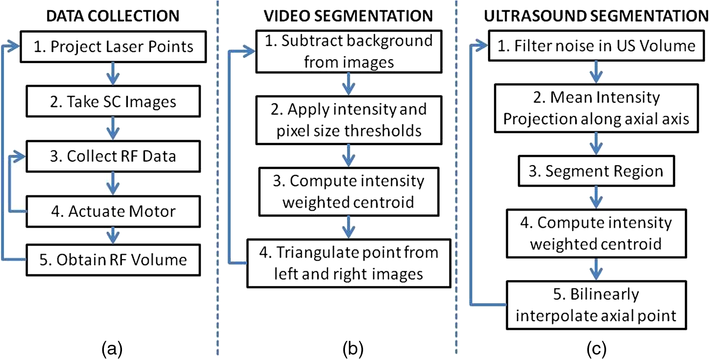
Each of our experiments was split into a data collection phase, a data processing phase, and a registration phase. The data collection phase outputted SC image pairs, five images for each camera, and a 3-D RF US volume for each projected laser spot. The data processing phase used the data and generates a 3-D SC point set and 3-D US point set. Finally, the registration phase used the two point sets to compute a coordinate transformation from the SC frame to the US frame. Figure 2(a) shows the experimental setup using the porcine liver phantom and an overlay of a US image representation using the inverse of the computed transformation.

Fig. 2

(a) Experimental setup and video overlay, (b) PA signal within an ultrasound (US) image.

Figure 3(a) shows the workflow of the data collection phase. First, a laser spot is projected onto the exposed surface of the ex vivo tissue, ex vivo fat, or synthetic material. It is important to emphasize that most of the laser energy from these laser spots are absorbed at the surface of the phantom. There are inaccuracies in SC spot triangulation if the laser spot is projected at or near the tissue or fat gelatin interface because the laser spots become irregularly shaped when projected onto clear materials. When projecting onto the fat, there was a significant reflectance and saturation due to its color. To reduce these effects, we placed laser goggles in front of the cameras, acting as a filter that modulates light intensities with varying wavelength-dependent optical densities. Second, several images were taken with each camera. The laser spot projected onto the phantom must be visible in at least one image per camera for triangulation to be possible. Our cameras had a faster capture rate than our laser’s repetition rate, so some of the frames were devoid of the laser signal. We exploit this during data processing. Steps 3 and 4 show that the 3-D US transducer motor actuation and RF data were intermittently collected from the DAQ device to scan and acquire the RF data of the volume of interest. The motor step size was 0.49 deg. The volume’s field of view varied among the experiments because the phantoms were of different sizes and several of them did not require as many slices to generate a volume that covered the entire phantom. The probe has a lateral length of 38.4 mm and the resulting PA images have a depth of 8 cm. A real-time implementation is feasible and an automatic process is in development. Currently, the manual process takes approximately $3\mathrm{s}/\mathrm{slice}$. This workflow was repeated for each of the laser spots.

Fig. 3

Workflow for (a) data collection, (b) SC segmentation, and (c) US segmentation.

From the data collection phase, we present the results showing that we can generate a PA point signal on the various phantoms using 532 nm, 1064 nm, or both. In each of these cases, the laser energy is mostly absorbed at the surface and the laser light does not interact with any medium other than air and the surface of the phantom. As we described, only a small amount of energy per pulse is required to generate a single PA spot and to localize it at the air–tissue interface. These are shown as a series of images similar to the one shown in Fig. 2(b). The size or location of the PA spot is unrelated between scenarios as parameters such as spot size or laser energy were different. Since we are displaying a 2-D slice from a 3-D volume, it is also possible that the displayed image does not contain the centroid of the PA signal.

The data processing phase involved the segmentation of the SC images into 3-D SC points, the segmentation of the 3-D RF US volume data into 3-D US points, and the computation of the transformation from the SC frame to the US frame.

Figure 3(b) shows the workflow for SC segmentation. For each camera, we picked a SC image with the laser spot and without the laser spot. Next, the background images without the laser spot were subtracted from the images with the laser spot. As we can see from Fig. 4(a), the laser spot is nearly segmented from the scene. We used an iris to decrease the beam size of the laser and the reflection from the iris results in the laser spot in the lower left. To compensate for this spot, we neglected an appropriate border on each image. We then applied an intensity and pixel size thresholds such that the laser spot is segmented out. These thresholds were selected based on the laser beam diameter and the phantom’s reflectance and are varied between the different scenarios. The thresholds were selected manually, but a method to automate threshold selection based on experimental parameters is in development. Next, we fitted an ellipse to the segmented region and computed the intensity-weighted centroid based on the pixels within the ellipse from the original image, resulting in the image shown in Fig. 4(b). Calibration files for our specific SC allowed us to triangulate the segmented point from each camera and to obtain a single 3-D point in the SC frame. In our current implementation, this step takes approximately 500 ms for each laser spot projection. This workflow was repeated for each laser spot projection.

Fig. 4

(a) Resulting image of US segmentation workflow steps 2, 3, and 4, (b) workflow for transformation, and (c) US and SC point cloud registered together.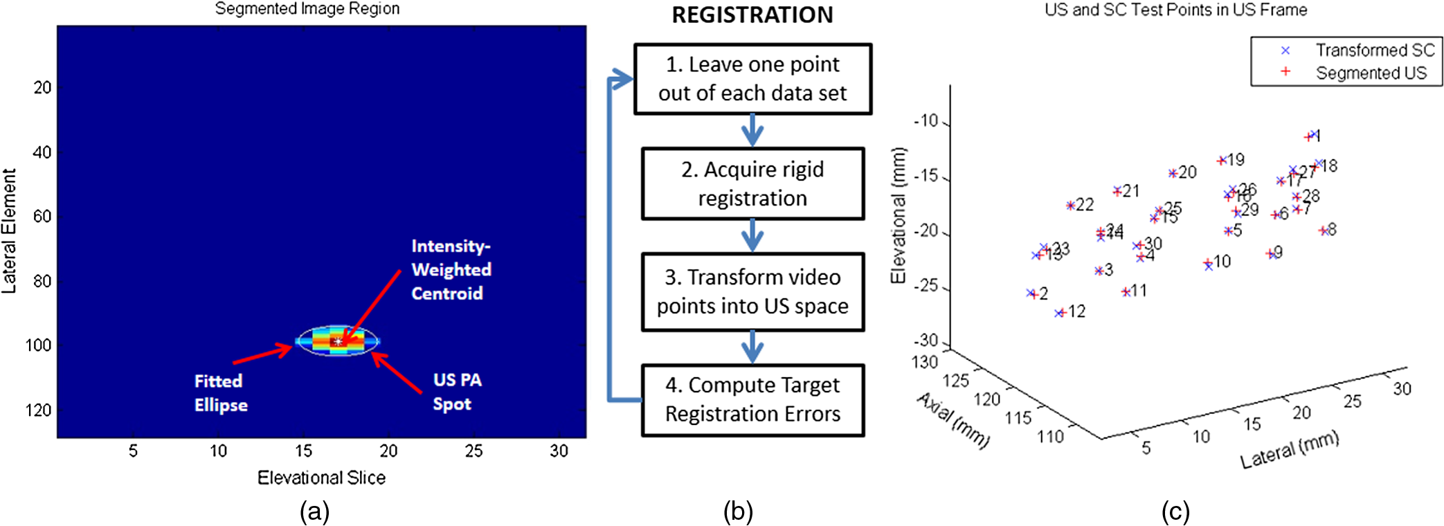

The workflow for the segmentation of the 3-D RF US volume is shown in Fig. 3(c). First, for each slice of a 3-D RF US volume, the RF data were beamformed using the $k$-wave toolbox¹⁶ in MATLAB. The dynamic range of the image was normalized with respect to the volume, and we applied a threshold to decrease the size of the PA signal seen in each volume. These thresholds ranged from 0.4 to 0.5. The size of the PA signal refers to the number of nonzero valued pixels, representing the PA signal after thresholding. A smaller size leads to a more compact representation of the PA signal, but it is also important to maintain the characteristic elliptical shape of the PA signal. Figure 2(b) shows a k-wave beamformed PA signal image. Beamforming requires approximately 140 ms for each PA image. Next, we projected the volume onto the lateral–elevational plane by taking the mean along each axial ray. An intensity and pixel size threshold were then applied to this image. These thresholds were selected in a similar fashion to the ones used for SC segmentation. An ellipse was fitted on the segmented region and an intensity-weighted centroid was computed resulting in lateral and elevational coordinates. Figure 5(a) is an example of this step showing the lateral–elevational image and the corresponding ellipse. As described earlier, the PA signal originated from the surface and any penetration into the surface. Since air cannot generate a PA signal in our setup, we conjecture that the high intensity pixels farthest away in the axial direction are from the surface. Thus, we obtained the axial coordinate corresponding with a lateral–elevational coordinate as the axial-most high intensity pixel. This step is particularly important because the penetration of the laser pulse was deeper for ex vivo tissue than the penetration for the synthetic phantom because the laser energy was not completely absorbed at the surface. We used bilinear interpolation to obtain axial coordinates between sampled points. These three coordinates were converted to 3-D US coordinates based on transducer specifications. The lateral coordinate combined with the lateral resolution of our US transducer results in the lateral coordinate in 3-D US space. The axial coordinate combined with the axial resolution represents a ray protruding from the US transducer, whereas the elevational coordinate relates to the angle in which this ray interacts with the first US image in the volume. Solving this geometry problem results in a 3-D US coordinate. The computation time for this process, not including beamforming, is correlated to the number of slices and field of view in each volume. Thus, the synthetic phantom required approximately $730\mathrm{ms}/\text{volume}$ and the other phantoms required approximately 570 ms. A 3-D RF US volume was acquired for each PA spot.

Fig. 5

Resulting images of video segmentation workflow for (a) step 1 and (b) step 3.

From the data processing phase, we present the localization accuracy of the US PA signal segmentation. In these results, we assume that the segmented SC points are the ground truth. For each US point set, we compute the distance between each pair of points. We compare the US distance of a particular pair of points with the distance between the same pair of SC points. The average of all differences for all point pairs is the recorded LE. These are reported in each of the lateral, axial, and elevational axes and the overall Euclidean distance for each experiment.

The transformation from the SC frame to the US frame was computed with the 3-D SC and 3-D US point sets as shown by the registration workflow in Fig. 5(b). Any registration method for computing the transformation between two 3-D point sets can be used. We used the coherent point drift algorithm²¹ in our experiments. One of the main reasons for using coherent point drift was that it allows for the data points to be missing from either dataset. An assumption that we have made is that every laser spot will be visible in the SC images and every PA signal will be visible in the US volume. This assumption was valid for our experiments but may not hold in the surgical setting due to SC or US transducer movement. Some of the points may lie outside the field of view of either the SC or the US transducer. The coherent point drift registration algorithm allowed us to acquire a registration as long as there were enough corresponding points in the SC images and the US volume. More experiments will be necessary to determine how many points are enough and if there will be any corresponding tradeoff in accuracy.

In Fig. 5(c), each SC point was independently used as a test point, whereas the rest of the points in the point set were used to transform the SC test point into the US domain. The figure shows the test SC point alongside its corresponding US point with a vector connecting the two. Our results from the registration workflow are shown as a series of target registration errors (TRE) computations in each of the lateral, axial, and elevational axes and the overall Euclidean distance for each experiment.

The transformation from the SC frame to the US frame was used to transform the 3-D SC points to the US frame for validation. The inverse transformation was used to display a representation of US image into the SC frame as shown in Fig. 2(a).

3.

Results

Three sets of results from various points in our experiment are presented: the ability to generate a PA point signal, a comparison of the point LEs in the SC and US domains, and registration error results.

The first set of results indicates that we can generate a PA point signal on a variety of materials using various energy levels or wavelengths. Table 1 specifies each of the five scenarios that we tried. Figure 6 shows the US images displaying a PA signal corresponding with each of the scenarios in Table 1.

Fig. 6

Sample PA images for (a) scenario 1, (b) scenario 2, (c) scenario 3, (d) scenario 4, and (e) scenario 5.

The second set of results includes the LEs of the PA points in scenarios 1 to 4 outlined in Table 2. Scenario 5 is not included because the 1064 nm wavelength light is invisible to the SC. This means that scenario 5 is not applicable to our experiments with the current design. The metric that we use is defined in Eq. (1). As mentioned previously, we compute the difference of the distance between a point pair in the US space versus the distance between a point pair in the SC space. This metric treats the SC points as the ground truth. The reported LE is the average of these differences over all point pairs for each experiment.

Table 2

Average LE results for experiments.

The registration results of our experiments on the synthetic phantom, the ex vivo liver phantom, the ex vivo kidney phantom, and the ex vivo fat phantom are validated using the TRE metric defined in Eq. (2). ${\mathrm{F}}_{\mathrm{SC}\_\mathrm{US}}$ is the transformation from the SC frame to the US frame and is computed with all of the SC and US points except for one. The TRE is the difference between the actual US test point and the transformed SC test point in the US frame.

$N$ is the number of points in a specific experiment and $N-1$ points is used to compute the transformation from the SC frame to the US frame. The remaining point is used as a test point to compute the TRE. This computation is repeated with each of the $N$ points as test points. Table 1 shows the average and standard deviation of the TRE results for the $N$ cases in the synthetic phantom, the ex vivo liver phantom, the ex vivo kidney phantom, and the ex vivo fat phantom experiments, respectively. Figure 7 shows the TRE results in a box-whisker plot.

Fig. 7

Box-whisker plot of TRE results for leave one out registration experiments.

4.

Discussion

As seen in Table 1, the energy densities used in the ex vivo liver and kidney experiments are close to or exceeding the MPE at that laser wavelength. These energy densities do not present a concern as we were not using the lowest possible energy density to generate the PA effect. Thus, energy density levels below the MPE threshold are quite feasible. Additionally, averaging multiple US PA images at a lower laser energy density can allow us to retain the same SNR at the expense of time. The energy density at 532 nm used in the ex vivo fat experiment does present a legitimate concern as it was an order of magnitude higher than the MPE. Fat is also the most likely material encountered in a realistic surgical setting as it covers the organ of interest and surgeons try to remove as little of it as possible. One situation where this method may benefit from an in vivo setup as opposed to an ex vivo setup is the presence of blood. At a wavelength of 532 nm, blood has a significantly higher absorption coefficient than fat.^22,23 It is therefore possibile that the blood on the fat surface be used to generate the PA signals as opposed to the fat itself. This would also mean that a much lower laser energy density is necessary.

As seen in Table 1, the energy density at 1064 nm used in the ex vivo fat experiment was beneath the MPE threshold. While we avoid energy density level concerns, this presents a situation where the SC used must be receptive to 1064 nm light. This is usually not the case as cameras typically have a visible range of 400 to 900 nm. A possible solution is to project a continuous wave, low power, visible laser that is coincident to the 1064 nm laser. However, this solution presents a new source of error as it may be difficult to achieve coincidental points. Another possible solution is to use a wavelength that is within the visible range of typical cameras yet has a higher absorption coefficient for fat than that observed at a wavelength of 532 nm.

The results in Table 2 imply that the US PA spots are being localized fairly accurately. The average and standard deviation of the difference in distance between all point pairs in the US and SC domain are submillimeter for each experimental scenario. These errors are in line with the point source LEs for typical SC systems.^5,6 Future studies for determining the LE may require a more accurate representation of ground truth data. A possible study is to project the laser spots on specific known locations of the phantom.

At the level of error measurements shown in Table 3, it is likely that the calibration of the SC system is a significant contributor. Optical markers can be tracked at submillimeter accuracy,^5,6 so this error is usually negligible in comparison with the approximate 3 mm errors from calibration.^5,6,7 Since our results were 0.56, 0.42, 0.38, and 0.85 mm errors, respectively, the SC system’s error became significant. We used a custom SC system, so its errors were also likely greater than a commercial SC system.

Table 3

Average TRE results for leave one out registration experiments.

From the experimental results shown in Table 3 and Fig. 7, it can be seen that our system achieved submillimeter TRE measurements for each of our experimental scenarios with different phantoms. We wish to highlight that these results are significantly better than the overall registration errors of approximately 1.7 to 3 mm for artificial phantoms and approximately 3 to 5 mm for tissue^3,4,9,10 presented in literature. There are several differences in the results between each scenario. First, the synthetic phantom had a larger Euclidean error than the ex vivo liver and ex vivo kidney phantoms almost entirely due to the elevational error. This was likely due to the larger field of view in the synthetic phantom experiment as well as normal variation across experiments. More experiments must be performed to obtain an average error across multiple experiments. The ex vivo fat experiment had noticeably worse results in both the mean and standard deviation in each direction and the Euclidean norm. A possible reason for this is the light delivery system. To achieve the energy density necessary to generate a PA signal on fat, we needed to focus our laser beam. Our setup was such that the focusing of the laser beam was not uniform across all points. As mentioned before, laser goggles were also placed in front of the SC for this particular experiment. These two circumstances differ from the other scenarios and may have introduced inconsistencies in the SC or US point sets. Another possibility may be the smaller sample size of this experiment compared to the rest.

There are several considerations when discussing this system’s deployment in our intended applications of laparoscopic tumor resections. The first is the placement of the transducer. In our experiments, we used a relatively large 3-D US transducer that would be difficult to place inside the body during a laparoscopic procedure. However, the transducer is often placed externally^3,10 in these procedures, so the size of the probe is not an issue. Naturally, there are disadvantages of placing the transducer externally and farther from the region or organ of interest. The SNR of US images degrades as the depth increases, which would likely lead to errors in localizing fiducials or, in our case, the PA signal. However, since the PA signal only has to travel in one direction, as opposed to traditional US, our PA images will have better quality than US images of equivalent depth.

Another issue with our 3-D US transducer was the acquisition speed. There are certain applications where an acquisition speed of a volume per several seconds is sufficient, but a real-time implementation would require a higher rate. We anticipate using 2-D array US transducers for a real-time implementation. These transducers would provide acquisition rates of 50 to $1000\text{volumes}/\mathrm{s}$.^24,25 These 2-D array transducers could also be fairly small and placed closer to the region of interest.

A third issue deals with the laser delivery system. As shown in our experimental setup, a laser would have to be fired at the organ in free space. This occurrence is unlikely in practical situations. We are developing a fiber delivery tool that will allow us to safely guide the laser beam into the patient’s body. This tool will also be able to project concurrent laser spots, greatly enhancing our registration acquisition rate.

The computation times shown throughout Secs. 2 and 3 still require some optimization for this method to become real-time at a reasonable refresh rate. The most obvious areas for improvement are data collection and PA image beamforming. The data collection phase can be improved dramatically with two changes. First of all, automated data collection as opposed to manual data collection would theoretically bring the data collection to the laser system pulse rate, which in our case is 10 Hz. The second issue would be the laser delivery system described above. Processing a single volume as opposed to a volume for each PA signal will greatly decrease computation time. PA beamforming computational cost is similar to conventional and current B-mode beamforming methods. Therefore, we do not anticipate technical or computational challenges to the implementation of real-time PA beamforming methods.

There are several factors that will affect this system’s errors as we move from a bench-top setup to in vivo experiments. When our SC system is replaced with a stereo endoscopic camera, the errors may increase because our SC system has a larger disparity due to the shorter distance between the two cameras in a stereo endoscopic camera. The disparity of a SC system directly affects the error in triangulating points found in each image into a 3-D point. Further work will be done to quantify the effects of this change. Also, the errors were reported based on surface points. Since the region of interest is often subsurface, our reported TRE will be biased for subsurface target errors. We believe that the bias will be fairly small since the PA spots are being detected in the same modality as any subsurface regions. Another factor is the effect of imaging a different medium using US. US images are generally reconstructed using a single speed of sound even though an image can contain multiple mediums with multiple speeds of sounds. There is significant variance in the speed of sounds in the phantoms that we used as ex vivo tissue and gelatin have different speed of sounds. This heterogeneity affects the axial scaling of the US image, but this is a problem that any US application must deal with.

5.

Conclusion

We have proposed an innovative 3-D US-to-video direct registration medical tracking technology based on PA markers and demonstrated its feasibility on multiple ex vivo tissue phantoms. In this paper, we showed the ability to generate a PA signal on multiple ex vivo tissue phantoms in various scenarios and PA spot LEs rivaling point source LEs found in SC systems. The TRE results have been shown to have higher accuracy than state of the art surgical navigation systems. Future work will include the development of a fiber delivery tool, spot finding algorithms to support concurrent spot projection, and subsequent in vivo animal experiments. Integration of this direct registration method into laparoscopic or robotic surgery environments will also be a point of emphasis.