Phantoms for diffuse optical imaging based on totally absorbing objects, part 1: basic concepts

Fabrizio Martelli; Antonio Pifferi; Davide Contini; Lorenzo Spinelli; Alessandro Torricelli; Heidrun Wabnitz; Rainer Macdonald; Angelo Sassaroli; Giovanni Zaccanti

doi:10.1117/1.JBO.18.6.066014

18 June 2013 Phantoms for diffuse optical imaging based on totally absorbing objects, part 1: basic concepts

Fabrizio Martelli, Antonio Pifferi, Davide Contini, Lorenzo Spinelli, Alessandro Torricelli, Heidrun Wabnitz, Rainer Macdonald, Angelo Sassaroli, Giovanni Zaccanti

Author Affiliations +

Journal of Biomedical Optics, Vol. 18, Issue 6, 066014 (June 2013). https://doi.org/10.1117/1.JBO.18.6.066014

Abstract

The design of inhomogeneous phantoms for diffuse optical imaging purposes using totally absorbing objects embedded in a diffusive medium is proposed and validated. From time-resolved and continuous-wave Monte Carlo simulations, it is shown that a given or desired perturbation strength caused by a realistic absorbing inhomogeneity of a certain absorption and volume can be approximately mimicked by a small totally absorbing object of a so-called equivalent black volume (equivalence relation). This concept can be useful in two ways. First, it can be exploited to design realistic inhomogeneous phantoms with different perturbation strengths simply using a set of black objects with different volumes. Further, it permits one to grade physiological or pathological changes on a reproducible scale of perturbation strengths given as equivalent black volumes, thus facilitating the performance assessment of clinical instruments. A set of plots and interpolating functions to derive the equivalent black volume corresponding to a given absorption change is provided. The application of the equivalent black volume concept for grading different optical perturbations is demonstrated for some examples.

1. Introduction

The investigation of the human body by diffusely propagated light is a highly appealing quest due to the intrinsic noninvasiveness of light at low power and the wealth of information carried by absorption (related to chemical composition) and scattering (linked to microstructure). Thus, a range of different applications have been devised and initially tested in clinics, such as optical mammography for the detection of breast lesions,¹^–³ monitoring of neoadjuvant chemotherapy,⁴ assessment of breast density as a cancer risk factor,⁵ functional imaging of the brain,⁶^–⁸ monitoring of blood perfusion and oxygenation in the injured brain,⁹ muscle oximetry,¹⁰ studies of epilepsy,¹¹^,¹² and investigation of bone and joint pathologies,¹³ just to cite same major examples.

Recently, the compelling need for standardization and quality assessment of diffuse optics instruments has been pointed out as a key requirement for the translation of the optical tools to effective clinical use.¹⁴ Indeed, the large variety of techniques and instruments, the diverse nature of clinical problems as well as the need of advanced theoretical modeling to extract clinically relevant parameters from the measurements demand some clearly identified and shared procedures to test and validate the optical systems. Common standardization tools help in comparing results obtained in different clinical studies, permit the grading of different instruments or subsequent upgrades of the same system, address the research—particularly at the industrial level—toward those parameters that best match the clinical needs. The work toward standardization requires, on one hand, the definition of shared protocols, identifying the key physical quantities to be measured and the procedures for their assessment¹⁴^–¹⁸ and, on the other hand, the description and production of phantoms mimicking some paradigmatic in vivo problems. For those problems that concern the protocols, several successful multilaboratory attempts have been initiated at the European Union (EU) level—fostered by EU-funded projects—such as the MEDPHOT protocol for the assessment of diffuse optics instruments on homogeneous media¹⁵ or, more recently, for characterization of time-domain brain imagers, the Basic Instrumental Performance protocol¹⁶ as well as the nEUROPt protocol,¹⁷ the latter being related to localized absorption changes.

Several studies have been focused on the design of tissue phantoms over the last decades, with the contribution¹⁹^–²⁶ of many groups (see Ref. 27 for a recent review). For homogeneous liquid phantoms, a high accuracy in characterization of Intralipid and India ink has been achieved.²⁸^,²⁹ A recent multicenter study of nine different laboratories³⁰ resulted in common mean values for the intrinsic scattering of Intralipid and the intrinsic absorption of ink with an associated uncertainty of 1% and 2%, respectively. Solid homogenenous phantoms can also be accurately characterized and are commercially available with a stated uncertainty of about 11% for the absorption coefficient, $μ_{a}$ , and about 7% for the reduced scattering coefficient, $μ_{s}^{'}$ (Ref. 31). Conversely, the production of inhomogeneous phantoms—mimicking, for instance, a focal activation in the brain cortex or a tumor mass within the breast—is more challenging, due to the added complexity of fabricating the structure by solid–solid, solid–liquid, or liquid–liquid phases. The possible artifacts due to the solid–liquid interface, or to the material layer separating two liquid phases, raise concern. Also, the large number of possible combinations, involving not only the host medium optical properties but also the location of source and detector, size, position, and properties of the local inhomogeneities, together with the source–detector arrangement, add to the overall complexity of the problem. Finally, the construction of dynamic phantoms, with the chance to easily and quickly vary phantom parameters, is a further need.

Just to quote a few examples to understand the complexity of inhomogeneous phantoms, the use of agar or agarose was proposed to create solid inclusions starting from Intralipid and ink dilutions,²¹^,³² yet with some criticalities, like scattering reduction produced by agar requiring proper compensation, diffusion of chromophores into and from the inhomogeneity, complex fabrication procedure, and fragility in handling and conservation. The use of transparent tubes, even with thin walls, can produce artifacts because of light-guiding effects. Solid inhomogeneities made, for example, of resin are definitely practical for use in liquid environments, yet refractive-index mismatch and potentially not-perfect matching of scattering properties could be an issue.³³

In this paper, we will show that the effect of a localized variation of the absorption coefficient within a finite volume can be adequately reproduced using a small totally absorbing object with a proper volume (equivalence relation). This concept can be useful in two ways. First, it can be exploited to design realistic inhomogeneous phantoms using a set of black objects with different volumes. Further, it permits one to grade physiological or pathological changes on a reproducible scale of black-equivalent volumes, thus facilitating the performance assessment of clinical instruments.

Although totally absorbing objects (e.g., black PVC cylinders) have already been used in diffuse spectroscopy experiments,³⁴^–³⁸ their far-ranging equivalence to realistic absorption inhomogeneities has never been thoroughly investigated. Also, the effect of a totally absorbing volume has never been quantified. The present study encompasses both continuous wave (CW) and time-resolved measurements, with an obvious extension to the frequency-domain case.

In the following, we will first present the equivalence relation from basic theoretical inferences (Sec. 2) and the methods used (Sec. 3). Then we will investigate its applicability with Monte Carlo (MC) simulations spanning a wide range of possible scenarios (Sec. 4). We will provide a set of look-up plots and interpolating functions to derive the equivalent black volume (EBV) yielding the same effect as a realistic absorption object (Sec. 5). Finally, an example of the use of EBV for grading different optical perturbations will be shown (Sec. 6).

This work will be followed by a companion paper where the EBV approach is actually implemented for the construction of simple and highly versatile inhomogeneous phantoms. All specifications on the phantom construction will be provided, together with an extensive numerical and experimental validation. It is worth mentioning that the EBV concept and the related phantom forms an essential basis of the nEUROPt protocol¹⁷ for the Performance Assessment of Time-Domain Optical Brain Imagers. This protocol has been agreed to by a consortium of 17 partners all over Europe and has been applied to the clinical brain imagers and additional laboratory instruments developed by four groups of this consortium.

2. Equivalence Relation Between Black and Realistic Inclusions: Formulation within the Diffusion Theory

Biological tissue is a heterogeneous medium and several imaging applications to tissue, such as the case of a focal activation in the brain cortex or the case of a tumor mass within the breast, are related to the detection of an absorption variation confined within a certain volume in such a medium. In this section, we refer to a diffusive medium in which an absorption variation takes place inside a localized volume of the medium (see Fig. 1 for a schematic).

Fig. 1

Schematic of an absorbing inclusion inside a diffusive medium.

When a small single absorbing object is placed inside a diffusive medium (homogeneous or heterogeneous), it is possible to formulate an equivalence relation so that a small and completely black object can give the same result for the perturbation as that for a larger object with only moderate absorption change. By small object we mean an absorbing inclusion of volume $V_{i}$ placed in a position $r_{0}$ inside the diffusive medium so that the unperturbed Green function is nearly constant over $V_{i}$ . The time-dependent fluence rate can be expressed as³⁹

Eq. (1)

Φ (r, t) = Φ^{0} (r, t) - \int_{V_{i}} d r^{'} Δ μ_{a} (r^{'}) \int_{- \infty}^{+ \infty} d t^{'} Φ (r^{'}, t^{'}) G (r, r^{'}, t, t^{'}),

where

Φ

is the perturbed fluence,

Φ^{0}

is the unperturbed fluence,

G

is the unperturbed Green function,

Δ μ_{a}

is the absorption variation of the object with respect to the background,

r

is the field point, and

r^{'}

denotes any point inside

V_{i}

. This integral equation can be written in any geometry (slab, semi-infinite medium, cylinder, etc.) and for any distribution of the optical properties of the background medium. The simplest and most approximated evidence of the equivalence relation can be noticed within the Born approximation, i.e., assuming

| Φ - Φ^{0} | ≪ Φ^{0}

, so that Eq. (1) becomes

Eq. (2)

Φ (r, t) = Φ^{0} (r, t) - \int_{V_{i}} d r^{'} Δ μ_{a} (r^{'}) \int_{- \infty}^{+ \infty} d t^{'} Φ^{0} (r^{'}, t^{'}) G (r, r^{'}, t, t^{'}) .

Equation (2) directly yields the Green function of the perturbed medium once the Green function of the unperturbed medium is known. Equation (2) can be written, assuming the unperturbed fluence and the Green’s function constant over

V_{i}

, in the following form:

Eq. (3)

Φ (r, t) = Φ^{0} (r, t) [1 - P (r, r_{0}, μ_{s}^{'}, t) Q (Δ μ_{a}, V_{i})],

where

Eq. (4)

P (r, r_{0}, μ_{s}^{'}, t) = Φ^{0} {(r, t)}^{- 1} \int_{- \infty}^{+ \infty} d t^{'} Φ^{0} (r_{0}, t^{'}) G (r, r_{0}, t, t^{'})

Eq. (5)

Q (Δ μ_{a}, V_{i}) = \int_{V_{i}} d r^{'} Δ μ_{a} (r^{'}) .

Q (Δ μ_{a}, V_{i})

measures the strength of the object, and when

μ_{a}

is constant over

V_{i}

, it is

Q = Δ μ_{a} V_{i}

. The time-dependent function

P

depends on the center of the absorbing object,

r_{0}

, on the reduced scattering coefficient of the background medium,

μ_{s}^{'}

, and on the geometry of the surrounding medium, while for homogeneous media in term of absorption, it is independent of the absorption coefficient

μ_{a}

of the background since the Beer-Lambert attenuation factor

\exp (- μ_{a} v t)

is identical both for

Φ (r, t)

and for

Φ^{0} (r, t)

. By using the functions

P

and

Q

, the time-dependent contrast

C (t)

can be expressed as

Eq. (6)

C (t) = [Φ (t) - Φ^{0} (t)] / Φ^{0} (t) = P (r, r_{0}, μ_{s}^{'}, t) Q (Δ μ_{a}, V_{i}),

i.e., as the factorization of the function

P

describing the temporal shape of the perturbation and the term

Q

accounting for the intensity of the perturbation. Also, the time-dependent contrast is independent of

μ_{a}

. Equation (3) expresses the equivalence relation since equivalent perturbations in terms of time-dependent contrast may be produced by different absorbing inclusions. A similar procedure can be repeated for a CW source, leading to a similar expression for the CW contrast

Eq. (7)

C_{CW} = (Φ_{CW} - Φ_{CW}^{0}) / Φ_{CW}^{0} = P_{CW} (r, r_{0}, μ_{s}^{'}, μ_{a}) Q (Δ μ_{a}, V_{i}),

with the function

P_{CW} (r, r_{0}, μ_{s}^{'}, μ_{a})

describing the spatial shape of the perturbation. We stress that different from the time-dependent case, the dependence on

μ_{a}

in Eq. (7) cannot be factorized [see Eq. (4.22) of Ref. 39, that is, the expression of

Φ_{CW}^{0}

for the slab] and both

P_{CW}

and

C_{CW}

depend on the background absorption coefficient

μ_{a}

.

Paasschens and Hooft,³⁵ making use of an iterative procedure and by expressing $Φ$ for the frequency domain and for an infinite medium as a Neumann series, extended the validity of Eq. (3) beyond the Born approximation. In their proof, Eq. (3) holds exactly within the diffusion approximation and for small absorbing objects. Yet, it can accommodate even large values for the absorption of the inhomogeneities.

Within the range of validity of this approximation, we find that the relative perturbation depends only on the position of the object and on its strength, while the shape of the object and the precise distribution of the absorption inside the object are not important. Accordingly, a small and completely black object can give the same relative perturbation as a larger object, with only moderate absorption. The equivalence relation can also be summarized noting that, according to Eqs. (6) and (7), the shapes of the time-dependent relative perturbation, $C (t)$ , and of the CW relative perturbation, $C_{CW}$ , are independent of the intensity of the perturbation $Q$ .

When the diffusion equation cannot be applied because the inclusion is too close to the boundary, to the source, or to the detector, the validity of the equivalence relation needs to be checked. With this purpose, by using numerical solutions of the radiative transfer equation reconstructed with an MC code, in Sec. 4, we have investigated the validity of the equivalence relation beyond the diffusive regime. It is also worth stressing that a validation of this relation is also necessary because in those regions, such as black inclusions, where absorption is much higher than scattering, the diffusion approximation is not expected to hold. Although Paasschens and Hooft have derived an expression for the strength of the perturbation due to a small black sphere, their theory shows discrepancies compared with the results of MC simulations. For this reason, a validation of this relation is necessary in order to extend its use to general conditions of photon migration: Sec. 4 will be devoted to this purpose for the time domain and for the CW domain. The results presented in this section cover a wide range of possible geometrical scenarios.

3. Methods

3.1.

Monte Carlo Code

A perturbation MC code was used to simulate photon migration through absorbing objects placed inside turbid media,³⁹^–⁴¹ in order to have reference data for our investigations. The MC method provides a physical simulation of photon migration inside the medium. Thus solutions of the radiative transfer equation can be obtained without any need for simplifying assumptions. Therefore the solutions obtained can be used as a standard reference for validation of approximate theories. In particular, in Sec. 4, MC data have been used to investigate the validity of the equivalence relation beyond the diffusive regime of light propagation and in Sec. 5 MC data have been used for measuring the EBV of an absorbing object. The perturbation MC used to generate the data shown in Secs. 4 and 5, strictly speaking, is not an elementary MC code since it makes use of scaling relationships so that the temporal response, when scattering or absorbing inhomogeneities are introduced, can be evaluated in a short time from the results of only one simulation carried out for the homogeneous medium.³⁹^,⁴⁰ We stress that an elementary MC is not suitable for calculating, with enough good statistics, the effects of absorbing inhomogeneities like those considered in our investigation.

3.2.

Determination of the Equivalent Black Volume

The procedure we adopted to derive the volume of the totally absorbing sphere that is equivalent to a given realistic inclusion is based on the comparison of the temporal contrast produced by any target object (realistic or totally absorbing) to the one yielded by an arbitrarily chosen reference object (e.g., a totally absorbing sphere of $1 {mm}^{3}$ volume). The procedure is explained in Fig. 2. First, the temporal contrast $C (t)$ is calculated, both for the target and the reference objects, for a large set of geometries (locations of the inclusion), and for a given value of the background reduced scattering coefficient [ $C (t)$ does not depend on the background absorption]. The figure refers to a semi-infinite medium with $μ_{s}^{'} = 1 {mm}^{- 1}$ ; the source is at (0,0,0) and the receiver at (30,0,0) mm. The target object is a volume of $1000 {mm}^{3}$ with $Δ μ_{a} = 0.02 {mm}^{- 1}$ . The reference object is a totally absorbing sphere of $1 {mm}^{3}$ . The two plots in Fig. 2 display the contrast function $C (t)$ for the target (upper graph) and the reference (lower graph) object in a given geometry. It can be observed that the shape of the $C (t)$ functions is much the same in the two cases. Then, the area $A$ under the $C (t)$ distribution, $A = \int_{0}^{+ \infty} C (t) d t$ , is calculated for both objects and for all the source–detector positions with respect to the inclusion, obtaining a set of $A$ and $A_{0}$ values for the target and reference objects, respectively. Figure 2 shows an example of the set of $A$ (top table) and $A_{0}$ (middle table) values calculated for different choices of the lateral position $x_{i}$ (heading row of the tables) and of the depth $z_{i}$ of the object (left column of the tables). It is worth pointing out that the value of $A$ is not the contrast produced by the perturbation in a CW case. Although there is an integral over the photon traveling time $t$ , this is applied after dividing $Δ ϕ (t)$ for $ϕ (t)$ . Finally, the measure $m$ of the target object is derived as the average of the ratios $A / A_{0}$ (bottom table) of the two datasets. Thus, a realistic inclusion and a totally absorbing inclusion are equivalent if they yield the same measure $m$ with respect to the reference totally absorbing sphere. Other procedures to find the set of equivalent objects can be designed, yet all results presented in the following sections were obtained using the method described above.

Fig. 2

Explanation of the method used to quantify the measure of the perturbation $m = {〈 A / A_{0} 〉}_{x_{i} z_{i}}$ produced by a target inclusion with respect to a reference perturbation. The figure refers to a semi-infinite medium with $μ_{s}^{'} = 1 {mm}^{- 1}$ ; the source is at (0,0,0) and the receiver at (30,0,0) mm. The target object is a sphere of $1000 {mm}^{3}$ , with $Δ μ_{a} = 0.02 {mm}^{- 1}$ . The reference object is a totally absorbing sphere of $1 {mm}^{3}$ . The numbers $A$ and $A_{0}$ , which are reported in the tables, are the areas under the curve.

4. Validation of the Equivalence Relation

4.1.

Time-Resolved Case

The validity of the equivalence relation was tested on MC simulations by comparing the effect on the photon time-distribution produced by a realistic optical inhomogeneity or by its equivalent totally absorbing object determined with the method described in Sec. 3.2. Figure 3 (reflectance) and Fig. 4 (transmittance) show the plots of the relative temporal contrast $| C (t) |$ for a wide range of possible scenarios. In particular, four different realistic inhomogeneities with a volume of $V = 1000 {mm}^{3}$ , and four different values of $Δ μ_{a}$ (rows), are set at different depths (columns) ( $z_{i} / mm = 10, 15, 20$ for reflectance and $z_{i} / mm = 30, 25, 20$ for transmittance) and compared to the corresponding totally black inclusions, yielding a similar perturbation. The refractive index of the medium and of the external was 1.33. The plots display the contrast $C (t)$ for six different arrangements of source, inclusion, and detector. In Fig. 3, we have reflectance measurements at $ρ = 5 mm$ (R5) and $ρ = 30 mm$ (R30 and R30S): the inclusion is set midway for R5 and R30 ( $x_{i} / mm = 2.5$ , 15; $y_{i} = 0$ ) between source [placed at (0,0,0)] and detector [placed at (5,0,0) mm for R5 and at (30,0,0) mm for R30] and with an $x$ -offset with respect to the midpoint of 15 mm for R30S (that has $x_{i} = 30 mm$ , $y_{i} = 0$ ). In Fig. 4, we have transmittance measurements through a 4-cm thick slab (for three configurations of the inclusion), with the detector at $x = y = 0$ and $z = 40 mm$ : the inclusion is set on axis for ( $x_{i} = y_{i} = 0$ ) and off-axis with an $x$ -offset of 10 and 20 mm, respectively, i.e., $x_{i} = 10 mm$ , $y_{i} = 0$ and $x_{i} = 20 mm$ , $y_{i} = 0$ . Generally, there is a good correspondence between the shapes of the temporal profiles for the entangled couples of objects, which change consistently upon varying the measurement geometry of the depth of the inclusion, matching, in most cases, also the absolute value of the contrast. The main discrepancies arise for low absorbing perturbations (first row) or a shallower depth (first column). The discrepancy is easily explained for geometrical reasons. When the absorption contrast is low, the totally absorbing inclusion is small (e.g., $5 {mm}^{3}$ ); thus fewer photon trajectories are intercepted by the black object as compared to the much larger ( $1000 {mm}^{3}$ ) realistic perturbation. Moreover, this difference is more marked for shallower objects. Transmittance measurements with the inhomogeneity near the axis are more affected by this discrepancy since, for objects nearer to the source or to the detector, the strong reduction in size of the perturbation has a marked effect on the interception of photon trajectories.

Fig. 3

Monte Carlo comparisons between the time-resolved reflectance contrast due to a realistic absorption change $Δ μ_{a}$ within a volume of $1000 {mm}^{3}$ (dotted curves) and that of an equivalent black sphere $V_{black}$ (solid curves). A semi-infinite medium with $μ_{s}^{'} = 1 {mm}^{- 1}$ and refractive index equal to 1.33 is considered. Four realistic inhomogeneities with different values of $Δ μ_{a}$ (rows) were positioned at increasing depths $z_{i} / mm = 10$ , 15, 20 (columns) and compared to the equivalent black inclusions. The plots display the relative contrast $| C (t) |$ for three different arrangements of source, detector, and inclusion, namely reflectance measurements at $ρ = 5 mm$ (R5) and $ρ = 30 mm$ (R30) with the inclusion set midway ( $x_{i} / mm = 2.5$ , 15; $y_{i} = 0$ ) between source [placed at (0,0,0)] and detector. The last case (R30S) refers to $ρ = 30 mm$ with an $x$ -offset of 15 mm with respect to the midplane, i.e., $x_{i} = 30 mm$ , $y_{i} = 0$ . The results are independent of $μ_{a}$ .

Fig. 4

Monte Carlo comparisons between the time-resolved transmittance contrast due to a realistic absorption change $Δ μ_{a}$ within a volume of $1000 {mm}^{3}$ (dotted curves) and that of an equivalent black sphere $V_{black}$ (solid curves). A slab 40 mm thick with $μ_{s}^{'} = 1 {mm}^{- 1}$ and refractive index equal to 1.33 is considered. Four realistic inhomogeneities with different values of $Δ μ_{a}$ (rows) are set at decreasing depths $z_{i} / mm = 30$ , 25, 20 (columns) and compared to the equivalent black inclusions. The plots display the relative contrast $| C (t) |$ for three different arrangements of the inclusion, namely transmittance measurements on-axis ( $x_{i} = y_{i} = 0$ ) and off-axis, with an $x$ -offset of 10 mm and of 20 mm, with the source placed at (0,0,0) and the detector placed at (0,0,40) mm. The results are independent of 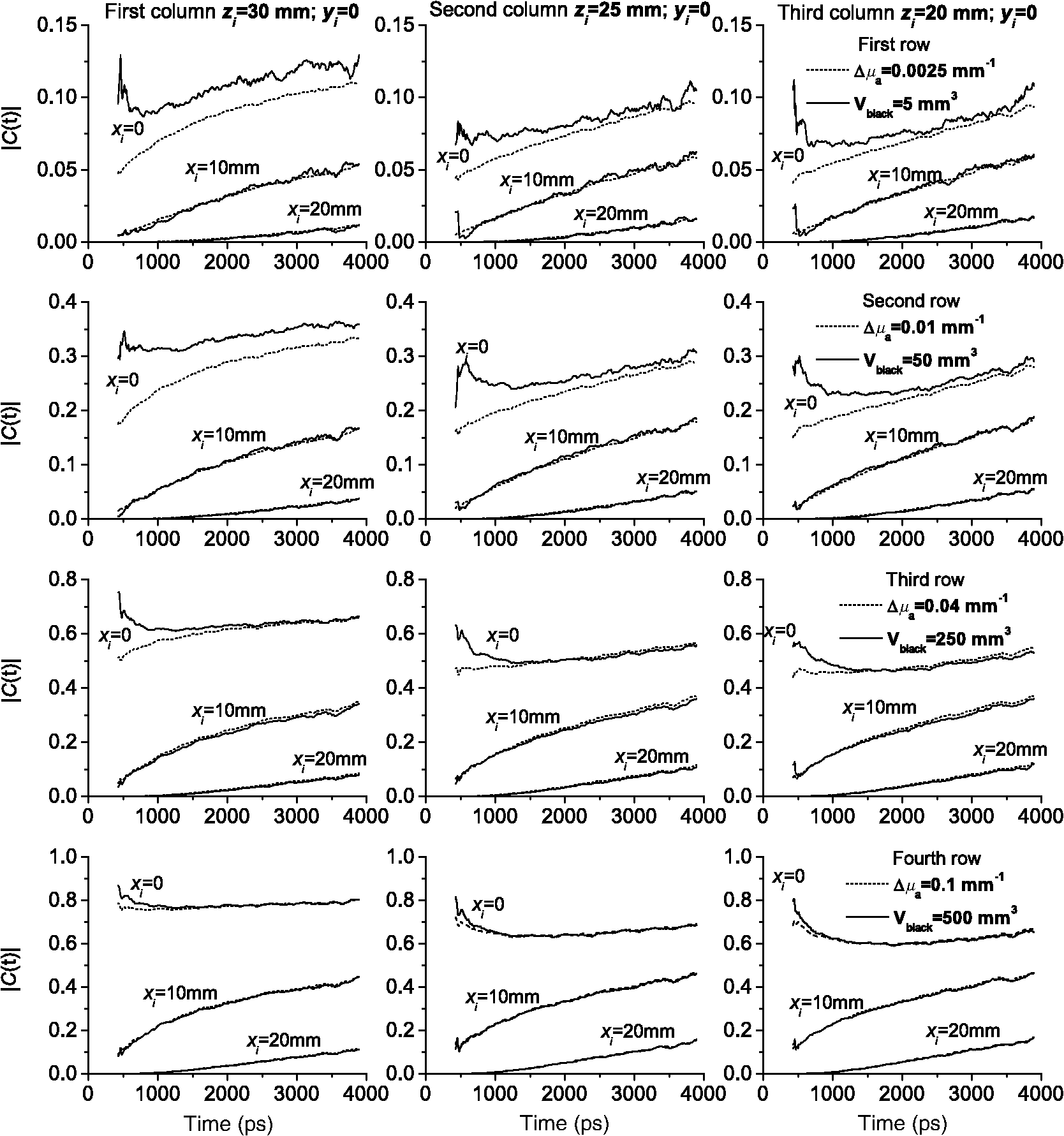$μ_{a}$ .

4.2.

Continuous Wave Case

In Sec. 2, we pointed out that $C (t)$ is rigorously independent of the background absorption. Conversely, in the CW domain, both the $P_{CW}$ function and the CW contrast depend on $μ_{a}$ , and the equivalence relation must also be validated against different choices of $μ_{a}$ . Figures 5 and 6 show the plots of the relative contrast $C_{CW}$ as a function of the absorption coefficient of the background $μ_{a}$ for the same four couples of realistic/black inhomogeneities (rows) set at several depths $z$ (columns) and the six geometries considered in Figs. 3 and 4. Overall, there is a generally good agreement between the black and the realistic perturbations, with largest discrepancies for the less-absorbing and shallower objects. Discrepancies are larger for larger values of $μ_{a}$ .

Fig. 5

Monte Carlo comparisons between the CW reflectance contrast due to a realistic $Δ μ_{a}$ within a volume of $1000 {mm}^{3}$ (dotted curves) and that of an equivalent black sphere $V_{black}$ (continuous curves). The data are plotted versus the absorption coefficient $μ_{a}$ of the background. A semi-infinite medium with $μ_{s}^{'} = 1 {mm}^{- 1}$ and refractive index equal to 1.33 is considered. Four realistic inhomogeneities with different values of $Δ μ_{a}$ (rows) were positioned at increasing depths $z_{i} / mm = 10$ , 15, 20 (columns) and compared to the corresponding totally black inclusions. The plots display the relative contrast $| C_{cw} |$ for three different arrangements of source and detector, namely reflectance measurements at $ρ = 5 mm$ (R5) and $ρ = 30 mm$ (R30) with the inclusion set midway ( $x_{i} / mm = 2.5$ , 15; $y_{i} = 0$ ) between source [placed at (0,0,0)] and detector. The last case with the perturbation set off-axis with an $x$ -offset of 15 mm with respect to the midpoint is for $ρ = 30 mm$ (R30S).

Fig. 6

Monte Carlo comparisons between the CW transmittance contrast through a slab due to a realistic $Δ μ_{a}$ within a volume of $1000 {mm}^{3}$ (dotted curves) and that of an equivalent black sphere $V_{black}$ (continuous curves). The data are plotted versus the absorption coefficient $μ_{a}$ of the background. A slab 40 mm thick with $μ_{s}^{'} = 1 {mm}^{- 1}$ and refractive index equal to 1.33 is considered. Four realistic inhomogeneities with different values of $Δ μ_{a}$ (rows) are set at decreasing depths $z_{i} / mm = 30$ , 25, 20 (columns) and compared to the corresponding totally black inclusions. The plots display the relative contrast $| C_{cw} |$ for three different arrangements of the inclusion, namely transmittance measurements on-axis ( $x_{i} = y_{i} = 0$ ) and off-axis with an $x$ -offset of 10 and 20 mm, with the source placed at (0,0,0) and the detector placed at (0,0,40) mm.

All simulations shown above were obtained for a background scattering coefficient $μ_{s}^{'} = 1 {mm}^{- 1}$ . For a different choice of $μ_{s}^{'} = 1 {mm}^{- 1}$ , a similar pattern is obtained, yet with different values of the totally absorbing inclusion.

Both for the time-resolved and the CW case, the discrepancy between the couples of objects is reduced for a lower volume (e.g., $500 {mm}^{3}$ ) of the realistic inhomogeneity (data not shown). Generally speaking, for a given $μ_{s}^{'}$ , the equivalence relation identifies—within the set of all possible (confined) absorption inhomogeneities—subclasses of equivalent objects producing the same effect. Each subclass contains only one totally absorbing spherical inclusion but an infinite variety of absorption inhomogeneities with different combinations of $Δ μ_{a}$ , volume, and shape. Thus, the equivalence relation can also be used to find matches between absorption inhomogeneities of different size.

5. Equivalent Black Volume

Since any realistic absorption perturbation—as far as the equivalence relation holds true—can be described by its equivalent totally absorbing inclusion, it is possible to use the volume of this inclusion as a measure of the perturbation. It is important to note that, within the same assumption, the equivalent volume is approximately the same, independent of the source–detector location, of the position of the perturbation, of $μ_{a}$ , while it changes for a different $μ_{s}^{'}$ . We first define a unitary EBV as

1 EBV = totally absorbing sphere of volume = 1 {mm}^{3} .

The EBV of any perturbation (both realistic and totally absorbing) is then expressed as the volume (measured in

{mm}^{3}

) of the equivalent totally absorbing sphere yielding the same effect under the same experimental conditions in terms of geometry (locations of the source, detector, and inclusion) and background optical properties. Figure 7 (left) summarizes the measure in EBV units for spherical realistic inhomogeneities with a volume of

1000 {mm}^{3}

as a function of their absorption (

Δ μ_{a}

). Three different choices of the background scattering coefficient (

μ_{s}^{'}

) are displayed, namely

μ_{s}^{'} = 0.5

(diamonds), 1 (circles), and

2 {mm}^{- 1}

(stars). The markers are EBV measurements obtained from MC results. The continuous dotted curves represent the interpolation of the simulated MC points using empirical interpolating functions. The use of these interpolating functions provides a tool for calculating the intensity of the realistic absorption perturbation of volume

1000 {mm}^{3}

equivalent to a certain black object of volume

V_{black}

. The interpolating function

Δ μ_{a} (V_{black})

used was a power law for small values of

V_{black}

(

< 30 {mm}^{3}

) and a polynomial for larger values of

V_{black}

Eq. (8)

Δ μ_{a} (V_{black}) = α {(V_{black})}^{β} (V_{black}) < 30 {mm}^{3} Δ μ_{a} (V_{black}) = \sum_{n = 0}^{6} C_{n} {(V_{black})}^{n} 30 {mm}^{3} < (V_{black}) < 600 {mm}^{3} .

The two different functions reflect the different dependence of

Δ μ_{a}

on

V_{black}

when

V_{black}

increases. The retrieved values of the coefficients have been summarized in Table 1, where the correlation coefficients obtained from the retrieval have also been shown. Figure 7 (right) displays the data at an enlarged scale, i.e., for

Δ μ_{a} < 0.01 {mm}^{- 1}

, to better visualize the behavior of small perturbations.

Fig. 7

The figure summarizes the measure in EBV units for spherical realistic inhomogeneities with a volume of $1000 {mm}^{3}$ as a function of their absorption ( $Δ μ_{a}$ ). Three different choices of the background $μ_{s}^{'}$ are displayed, namely $μ_{s}^{'} = 0.5$ (diamonds), 1 (circles), and $2 {mm}^{- 1}$ (stars). The markers are MC results, while the continuous dotted curves represent the interpolation of the MC simulated points using empirical interpolating functions. In (a) there is the full dataset, while in (b) there is the first part of the same data on an enlarged scale.

Table 1

Coefficients of the interpolating function of Eq. (8) retrieved using MC data for μs′=0.5, 1, and 2 mm−1. The correlation coefficient R is also shown.

Coefficients	$μ_{s}^{'} = 0.5 {mm}^{- 1}$	$μ_{s}^{'} = 1 {mm}^{- 1}$	$μ_{s}^{'} = 2 {mm}^{- 1}$	$R$
$α$	1.07E-3	9.34E-4	7.03E-4	0.999
$β$	6.59E-1	6.05E-1	5.56E-1	0.999
$C_{0}$	4.15E-3	2.91E-3	1.93E-3	1
$C_{1}$	2.14E-4	1.58E-4	9.58E-5	1
$C_{2}$	$- 5.92 E - 7$	$- 4.01 E - 7$	$- 1.80 E - 7$	1
$C_{3}$	2.66E-9	1.85E-9	7.62E-10	1
$C_{4}$	$- 5.28 E - 12$	$- 3.36 E - 12$	$- 9.28 E - 13$	1
$C_{5}$	5.67E-15	3.26E-15	4.58E-16	1
$C_{6}$	$- 1.74 E - 18$	$- 6.14 E - 19$	4.20E-19	1

The concept of EBV makes possible the construction of realistic inhomogeneous phantoms for imaging purposes using a set of black objects with different volumes, By changing the volume, we change the intensity of the perturbation simulated in the optical phantom. Making use of this approach, the calibration of the optical properties of the inclusion is not necessary and the characterization of the absorption properties is based only on the equivalence relation. We stress that with this concept, the kind of perturbation that can be simulated is restricted to the condition $Δ μ_{a} > 0$ . When $Δ μ_{a} < 0$ , a totally absorbing object cannot be used to reproduce the same perturbation of a realistic inclusion. However, for small values of $Δ μ_{a}$ , the case $Δ μ_{a} < 0$ is complementary to the case $Δ μ_{a} > 0$ . Within the Born approximation, it is trivial to show that for an absorbing inclusion of fixed volume $C (Δ μ_{a}, t) = - C (- Δ μ_{a}, t)$ . For large values of $Δ μ_{a}$ , this property does not exactly hold true and some corrections need to be introduced. Finally, we also point out that within the range of validity of the equivalence relation, the results presented in this section are applicable both to the time domain and to the CW domain.

6. Examples of EBV Assessment

To better envision the potential use of the EBV measure, we report in Table 2 some examples of quantification of different perturbations for the particular applications of functional imaging of the brain and of optical mammography. Most of the results used referred to time-domain experiments. In particular, the table compares the measure of different optical perturbations, namely (a) a totally absorbing sphere of $1 {mm}^{3}$ volume, (b) an increase in absorption of $0.01 {mm}^{3}$ over a volume of $1000 {mm}^{3}$ , (c) an increase of oxy-( ${HbO}_{2}$ ) or deoxy-(Hb) hemoglobin of 100 nmol assessed at 800 nm, (d) the effect of a typical motor cortex activation assessed in vivo,⁴²^,⁴³ (f) the effect of a breast malignant lesion assessed in vivo.⁴^,⁵ All these perturbation effects can be compared in a quantitative way, since all of them can be graded using the EBV. In general, it is not necessary to specify the measurement geometry or the background optical properties, since the equivalence holds true within any combination of these parameters, yet within the limitations discussed above. However, in order to calculate the EBV corresponding to our target perturbation, the information on geometry and optical properties is required. This information is necessary for implementing the forward calculations used to generate the perturbations of the total absorbing objects to be matched to the measured perturbation. Therefore, for cases b, d, and f, the realistic volume of $1000 {mm}^{3}$ was assumed for calculating the EBV according to the previous section and a $μ_{s}^{'} = 1 {mm}^{- 1}$ was assumed for determining the EBV corresponding to cases b and c. Finally, for the last two cases, the calculation was carried out assuming a 15-mm depth (case d) and the lesion at midway in a thickness of 40 mm (case f). Truly, the assessment of the EBV for the in vivo data requires a rough estimate of both the inclusion depth and the background reduced scattering coefficient. In particular, the depth dependence is quite steep, leading to a substantial dependence of the estimated EBV on the assumed depth. Yet, once the EBV measure is derived, it can be compared to other in vivo results independent of the measurement system or geometry.

Table 2

Examples of absorption perturbations expressed as equivalent black volume.

Perturbation	EBV ( ${mm}^{3}$ )	Wavelength (nm)
${mm}^{3}$ totally absorbing sphere	1	—
$Δ μ_{a} = 0.01 {mm}^{- 1}$	50	—
nmol Hb	120	800
Motor task	$\approx 10$	830
Malignant breast lesion	$\approx 100$	635

The evaluation of the EBV units of a certain perturbation requires a forward solver for identifying the EBV. For producing the results presented in the previous sections, we have largely used an MC forward solver. The main limitation of the MC is the computation time since the evaluation of a certain perturbation should be preferably done in real time. For this reason, as an alternative to the MC, we have also developed an analytical forward solver based on a high-order perturbation theory⁴⁴^–⁴⁷ and on the equivalence relation. It is beyond the scope of this work, which is dedicated to the basic concepts, to provide details on this solver. What we want to stress is that the evaluation of the EBV units using the above-mentioned solver can be done in real time with any standard PC and with negligible differences compared to the results obtained with an MC solver.

The in vivo result presented above is just an example taken from the dataset collected in our laboratory and has no claim to represent an average or typical response. Rather, it is a realistic example presented to show the applicability of the approach and a rough idea on the quantification of an in vivo exercise. It would be worth applying this method in a systematic way to a collection of in vivo data to provide a quantitative description of in vivo activation to be used for tailoring phantom construction, or even to compare the results of different studies. These studies could also be greatly beneficial for the definition of standards, with the construction of an easily reproducible scale of “universal absorption inhomogeneities.” Similarly, the same exercise could be engaged for the quantification of breast lesions in optical mammography. Clearly, all this goes beyond the scope of the present paper.

7. Conclusions

In summary, we demonstrated that the equivalence relation, formulated in Sec. 2 within the diffusion theory, between a realistic and a totally absorbing inclusion has a rather broad range of validity (see Sec. 4). Its only limitation arises whenever there is a large discrepancy in size (as compared to the distance from the source–detector pair) between the realistic and the black inclusions. Practically this happens when the $Δ μ_{a}$ (between realistic inclusion and background) and the EBV are small and the inclusion is located quite shallowly and close either to the source or the detector. From Figs. 3, 4, 5, and 6 we notice that the discrepancies are larger in the transmittance when the inclusion is in front of the beam and in shallow positions. Except for these cases, discrepancies remain of the order of few percents. The complete overview provided with the presented figures can be used to select the optimal range where the equivalence relation holds with negligible error, or alternatively to account for the error due to its use. The range of absorption values where the equivalence relation shows larger approximations is also typical of some applications like breast tumors and brain functional imaging. Therefore, the use of the proposed approach with imaging instrumentation has to be carefully evaluated when the inclusion is in a shallow position. Finally, the equivalence relation can be used indifferently in the time domain and in the CW domain and, therefore, also in the frequency domain.

Based on the equivalence relation, we propose the construction of well-reproducible inhomogeneous phantoms where the defects are represented by totally absorbing objects, like black PVC cylinders, that produce the same effect of a realistic absorption inhomogeneity. Therefore, inhomogeneous phantoms for imaging purposes can be designed using a set of black objects with different volumes: the intensity of the perturbation simulated in the optical phantom can be changed by varying the volume of the black object used. Making use of this approach, the calibration of the optical properties of the defect is not necessary and the characterization of the absorption properties of the inclusion is based only on the equivalence relation. This approach is addressed to absorbing objects embedded in diffusive media and can be applied to design either liquid or solid phantoms.

Based on the equivalence relation, we have also introduced the EBV as a measure of a realistic perturbation defined as the volume of the equivalent totally absorbing inclusion that gives the same perturbation. In this way, physiological or pathological changes can be graded on a reproducible scale, thus facilitating the performance assessment of clinical instruments. Some interpolating functions derived from MC data have been provided in order to facilitate this task. Therefore, by using the functions of Eq. (8), it is possible to calculate the absorption variation $Δ μ_{a}$ of a realistic inclusion of volume $1000 {mm}^{3}$ that gives the same perturbation of a black volume. Finally, as an example of the measure in EBV units, we have expressed some perturbations for the particular applications of functional imaging of the brain and of optical mammography in this proposed units. These two realistic examples of perturbations (Table 2) can be represented in the range of about 10 to 100 EBV units and thus can be potentially reproduced with optical phantoms based on totally absorbing objects.

Acknowledgments

The research leading to these results has received funding from the European Community’s Seventh Framework Programme [FP7/2007-2013] under grant agreement No. FP7-HEALTH-F5-2008-201076. The research leading to these results has also received funding from LASERLAB-EUROPE (grant agreement No. 284464, European Community’s Seventh Framework Programme). This research is also supported by NIH Grant: R01-CA154774 and NSF Award: IIS 1065154.

References

1.

A. Torricelliet al., “Use of a nonlinear perturbation approach for in vivo breast lesion characterization by multiwavelength time-resolved optical mammography,” Opt. Express, 11 (8), 853 –867 (2003). http://dx.doi.org/10.1364/OE.11.000853 OPEXFF 1094-4087 Google Scholar

2.

P. Taroniet al., “Seven-wavelength time-resolved optical mammography extending beyond 1000 nm for breast collagen quantification,” Opt. Express, 17 (18), 15932 –15946 (2009). http://dx.doi.org/10.1364/OE.17.015932 OPEXFF 1094-4087 Google Scholar

3.

D. R. Leffet al., “Diffuse optical imaging of the healthy and diseased breast: a systematic review,” Breast Cancer Res. Treat., 108 (1), 9 –22 (2008). http://dx.doi.org/10.1007/s10549-007-9582-z BCTRD6 0167-6806 Google Scholar

4.

R. Choeet al., “Diffuse optical tomography of breast cancer during neoadjuvant chemotherapy: a case study with comparison to MRI,” Breast Cancer Res. Treat., 32 (4), 1128 –1139 (2005). http://dx.doi.org/10.1118/1.1869612 BCTRD6 0167-6806 Google Scholar

5.

P. Taroniet al., “Effects of tissue heterogeneity on the optical estimate of breast density,” Biomed. Opt. Express, 3 (10), 2411 –2418 (2012). http://dx.doi.org/10.1364/BOE.3.002411 BOEICL 2156-7085 Google Scholar

6.

E. Molteniet al., “Load-dependent brain activation assessed by time-domain functional near-infrared spectroscopy during a working memory task with graded levels of difficulty,” J. Biomed. Opt., 17 (5), 056005 (2012). http://dx.doi.org/10.1117/1.JBO.17.5.056005 JBOPFO 1083-3668 Google Scholar

7.

M. Buttiet al., “Effect of prolonged stimulation on cerebral hemodynamic: a time-resolved fNIRS study,” Med. Phys., 36 (9), 4103 –4114 (2009). http://dx.doi.org/10.1118/1.3190557 MPHYA6 0094-2405 Google Scholar

8.

T. Durduranet al., “Diffuse optics for tissue monitoring and tomography,” Rep. Prog. Phys., 73 (7), 076701 (2010). http://dx.doi.org/10.1088/0034-4885/73/7/076701 RPPHAG 0034-4885 Google Scholar

9.

M. N. Kimet al., “Noninvasive measurement of cerebral blood flow and blood oxygenation using near-infrared and diffuse correlation spectroscopies in critically brain-injured adults,” Neurocrit. Care, 12 (2), 173 –180 (2010). http://dx.doi.org/10.1007/s12028-009-9305-x NCEACB 1541-6933 Google Scholar

10.

R. A. De Blasiet al., “Cerebral and muscle oxygen saturation measurement by frequency-domain near-infra-red spectrometer,” Med. Biol. Eng. Comput., 33 (2), 228 –230 (1995). http://dx.doi.org/10.1007/BF02523048 MBECDY 0140-0118 Google Scholar

11.

B. J. SteinhoffG. HerrendorfC. Kurth, “Ictal near infrared spectroscopy in temporal lobe epilepsy: a pilot study,” Eur. J. Epilepsy, 5 (2), 97 –101 (1996). http://dx.doi.org/10.1016/S1059-1311(96)80101-4 1059-1311 Google Scholar

12.

L. Spinelliet al., “Multimodality fNIRS-EEG, fMRI-EEG and TMS clinical study on cortical response during motor task in adult volunteers and epileptic patients with movement disorders,” in Biomedical Optics, OSA Technical Digest, BM4A.1 (2012). Google Scholar

13.

A. H. Hielscheret al., “Frequency-domain optical tomographic imaging of arthritic finger joints,” IEEE Trans. Instrum. Meas., 30 (10), 1725 –1736 (2011). http://dx.doi.org/10.1109/TMI.2011.2135374 IEIMAO 0018-9456 Google Scholar

14.

J. HwangJ. C. Ramella-RomanR. Nordstrom, “Introduction: feature issue on phantoms for the performance evaluation and validation of optical medical imaging devices,” Biomed. Opt. Express, 3 (6), 1399 –1403 (2012). http://dx.doi.org/10.1364/BOE.3.001399 BOEICL 2156-7085 Google Scholar

15.

A. Pifferiet al., “Performance assessment of photon migration instruments: the MEDPHOT protocol,” Appl. Opt., 44 (11), 210414 (2005). http://dx.doi.org/10.1364/AO.44.002104 APOPAI 0003-6935 Google Scholar

16.

A. Wabnitzet al., “Assessment of basic instrumental performance of time-domain optical brain imagers,” Proc. SPIE, 7896 789602 (2011). http://dx.doi.org/10.1117/12.874654 PSISDG 0277-786X Google Scholar

17.

A. Wabnitzet al., “Performance assessment of time-domain optical brain imagers: the nEUROPt protocol,” in Biomedical Optics, OSA Technical Digest, BSu2A.4 (2012). Google Scholar

18.

C. H. Schmitzet al., “Instrumentation and calibration protocol for imaging dynamic features in dense-scattering media by optical tomography,” Appl. Opt., 39 (4), 6466 –6486 (2000). http://dx.doi.org/10.1364/AO.39.006466 APOPAI 0003-6935 Google Scholar

19.

M. FirbankD. T. Delpy, “A design for a stable and reproducible phantom for use in near infra-red imaging and spectroscopy,” Phys. Med. Biol., 38 847 –853 (1993). http://dx.doi.org/10.1088/0031-9155/38/6/015 PHMBA7 0031-9155 Google Scholar

20.

U. Sukowskiet al., “Preparation of solid phantoms with defined scattering and absorption properties for optical tomography,” Phys. Med. Biol., 41 (9), 1823 –1844 (1996). http://dx.doi.org/10.1088/0031-9155/41/9/017 PHMBA7 0031-9155 Google Scholar

21.

R. Cubedduet al., “A solid tissue phantom for photon migration studies,” Phys. Med. Biol., 42 (10), 1971 –1979 (1997). http://dx.doi.org/10.1088/0031-9155/42/10/011 PHMBA7 0031-9155 Google Scholar

22.

M. Lualdiet al., “A phantom with tissue-like optical properties in the visible and near infrared for use in photomedicine,” Lasers Surg. Med., 28 (3), 237 –243 (2001). http://dx.doi.org/10.1002/(ISSN)1096-9101 LSMEDI 0196-8092 Google Scholar

23.

J. C. Hebdenet al., “A soft deformable tissue-equivalent phantom for diffuse optical tomography,” Phys. Med. Biol., 51 (21), 5581 –5590 (2006). http://dx.doi.org/10.1088/0031-9155/51/21/013 PHMBA7 0031-9155 Google Scholar

24.

P. Di NinniF. MartelliG. Zaccanti, “Intralipid: towards a diffusive reference standard for optical tissue phantoms,” Phys. Med. Biol., 56 (2), N21 –N28 (2011). http://dx.doi.org/10.1088/0031-9155/56/2/N01 PHMBA7 0031-9155 Google Scholar

25.

A. E. Cerussiet al., “Tissue phantoms in multicenter clinical trials for diffuse optical technologies,” Biomed. Opt. Express, 3 (5), 966 –971 (2012). http://dx.doi.org/10.1364/BOE.3.000966 BOEICL 2156-7085 Google Scholar

26.

G. Lamoucheet al., “Review of tissue simulating phantoms with controllable optical, mechanical and structural properties for use in optical coherence tomography,” Biomed. Opt. Express, 3 (6), 1381 –1398 (2012). http://dx.doi.org/10.1364/BOE.3.001381 BOEICL 2156-7085 Google Scholar

27.

B. W. PogueM. S. Patterson, “Review of tissue simulating phantoms for optical spectroscopy, imaging and dosimetry,” J. Biomed. Opt., 11 (4), 041102 (2006). http://dx.doi.org/10.1117/1.2335429 JBOPFO 1083-3668 Google Scholar

28.

F. MartelliG. Zaccanti, “Calibration of scattering and absorption properties of a liquid diffusive medium at NIR wavelengths. CW method,” Opt. Express, 15 (2), 486 –500 (2007). http://dx.doi.org/10.1364/OE.15.000486 OPEXFF 1094-4087 Google Scholar

29.

L. Spinelliet al., “Calibration of scattering and absorption properties of a liquid diffusive medium at NIR wavelengths. Time-resolved method,” Opt. Express, 15 (11), 6589 –6604 (2007). http://dx.doi.org/10.1364/OE.15.006589 OPEXFF 1094-4087 Google Scholar

30.

L. Spinelliet al., “Inter-laboratory comparison of optical properties performed on Intralipid and India Ink,” BW1A.6 (2012). Google Scholar

31.

J. P. Bouchardet al., “Reference optical phantoms for diffuse optical spectroscopy. Part 1–Error analysis of a time resolved transmittance characterization method,” Opt. Express, 18 (11), 11495 –11507 (2010). http://dx.doi.org/10.1364/OE.18.011495 OPEXFF 1094-4087 Google Scholar

32.

L. Spinelliet al., “Experimental test of a perturbation model for time-resolved imaging in diffusive media,” Appl. Opt., 42 (16), 3145 –3153 (2003). http://dx.doi.org/10.1364/AO.42.003145 APOPAI 0003-6935 Google Scholar

33.

A. Puszkaet al., “Time-domain reflectance diffuse optical tomography with Mellin-Laplace transform for experimental detection and depth localization of a single absorbing inclusion,” Biomed. Opt. Express, 4 (4), 569 –583 (2013). http://dx.doi.org/10.1364/BOE.4.000569 BOEICL 2156-7085 Google Scholar

34.

D. A. Boaset al., “Scattering of diffuse photon density waves by spherical inhomogeneities within turbid media: analytic solution and application,” Proc. Natl. Acad. Sci., 91 (11), 4887 –4891 (1994). http://dx.doi.org/10.1073/pnas.91.11.4887 PMASAX 0096-9206 Google Scholar

35.

J. C. J. PaasschensG. W. Hooft, “Influence of boundaries on the imaging of objects in turbid media,” J. Opt. Soc. Am. A, 15 (7), 1797 –1812 (1998). http://dx.doi.org/10.1364/JOSAA.15.001797 JOAOD6 0740-3232 Google Scholar

36.

A. Takatsukiet al., “Absorber’s effect projected directly above improves spatial resolution in near infrared backscattered imaging,” Jpn. J. Physiol., 54 (1), 79 –86 (2004). http://dx.doi.org/10.2170/jjphysiol.54.79 JJPHAM 0021-521X Google Scholar

37.

A. Pifferiet al., “Time-resolved diffuse reflectance using small source-detector separation and fast single-photon gating,” Phys. Rev. Lett., 100 (3), 138101 (2008). http://dx.doi.org/10.1103/PhysRevLett.100.138101 PRLTAO 0031-9007 Google Scholar

38.

Q. Zhaoet al., “Functional tomography using a time-gated ICCD camera,” Biomed. Opt. Express, 2 (3), 705 –716 (2011). http://dx.doi.org/10.1364/BOE.2.000705 BOEICL 2156-7085 Google Scholar

39.

F. Martelliet al., Light Propagation Through Biological Tissue and Other Diffusive Media, SPIE Press, Bellingham, Washington (2010). Google Scholar

40.

A. Sassaroliet al., “Monte Carlo procedure for investigating light propagation and imaging of highly scattering media,” Appl. Opt., 37 (31), 7392 –7400 (1998). http://dx.doi.org/10.1364/AO.37.007392 APOPAI 0003-6935 Google Scholar

41.

C. K. Hayakawaet al., “Perturbation Monte Carlo methods to solve inverse photon migration problems in heterogeneous tissues,” Opt. Lett., 26 (17), 1335 –1337 (2001). http://dx.doi.org/10.1364/OL.26.001335 OPLEDP 0146-9592 Google Scholar

42.

D. Continiet al., “Multi-channel time-resolved system for functional near infrared spectroscopy,” Opt. Express, 14 5418 –5432 (2006). http://dx.doi.org/10.1364/OE.14.005418 OPEXFF 1094-4087 Google Scholar

43.

R. Reet al., “A compact time-resolved system for near infrared spectroscopy based on wavelength space multiplexing,” Rev. Sci. Instrum., 81 (11), 113101 (2010). http://dx.doi.org/10.1063/1.3495957 RSINAK 0034-6748 Google Scholar

44.

A. SassaroliF. MartelliS. Fantini, “Perturbation theory for the diffusion equation by use of the moments of the generalized temporal point-spread function. I. Theory,” J. Opt. Soc. Am. A, 23 (9), 2105 –2118 (2006). http://dx.doi.org/10.1364/JOSAA.23.002105 JOAOD6 0740-3232 Google Scholar

45.

A. SassaroliF. MartelliS. Fantini, “Perturbation theory for the diffusion equation by use of the moments of the generalized temporal point-spread function. II. Continuous-wave results,” J. Opt. Soc. Am. A, 23 (9), 2119 –2131 (2006). http://dx.doi.org/10.1364/JOSAA.23.002119 JOAOD6 0740-3232 Google Scholar

46.

A. SassaroliF. MartelliS. Fantini, “Higher-order perturbation theory for the diffusion equation in heterogeneous media: application to layered and slab geometries,” Appl. Opt., 48 (10), D62 –D73 (2009). http://dx.doi.org/10.1364/AO.48.000D62 APOPAI 0003-6935 Google Scholar

47.

A. SassaroliF. MartelliS. Fantini, “Perturbation theory for the diffusion equation by use of the moments of the generalized temporal point-spread function. III. Frequency-domain and time-domain results,” J. Opt. Soc. Am. A, 27 (7), 1723 –1742 (2010). http://dx.doi.org/10.1364/JOSAA.27.001723 JOAOD6 0740-3232 Google Scholar

CC BY: © The Authors. Published by SPIE under a Creative Commons Attribution 4.0 Unported License. Distribution or reproduction of this work in whole or in part requires full attribution of the original publication, including its DOI.

Citation Download Citation

Fabrizio Martelli, Antonio Pifferi, Davide Contini, Lorenzo Spinelli, Alessandro Torricelli, Heidrun Wabnitz, Rainer Macdonald, Angelo Sassaroli, and Giovanni Zaccanti "Phantoms for diffuse optical imaging based on totally absorbing objects, part 1: basic concepts," Journal of Biomedical Optics 18(6), 066014 (18 June 2013). https://doi.org/10.1117/1.JBO.18.6.066014

Published: 18 June 2013

Access the abstract

JOURNAL ARTICLE
12 PAGES

DOWNLOAD PAPER SAVE TO MY LIBRARY

GET CITATION

CITATIONS

Cited by 41 scholarly publications.

Explore citations on Lens.org

KEYWORDS

Absorption

Diffuse optical imaging

Monte Carlo methods

Sensors

Optical spheres

Scattering

Brain

1.

Introduction

2.

Equivalence Relation Between Black and Realistic Inclusions: Formulation within the Diffusion Theory