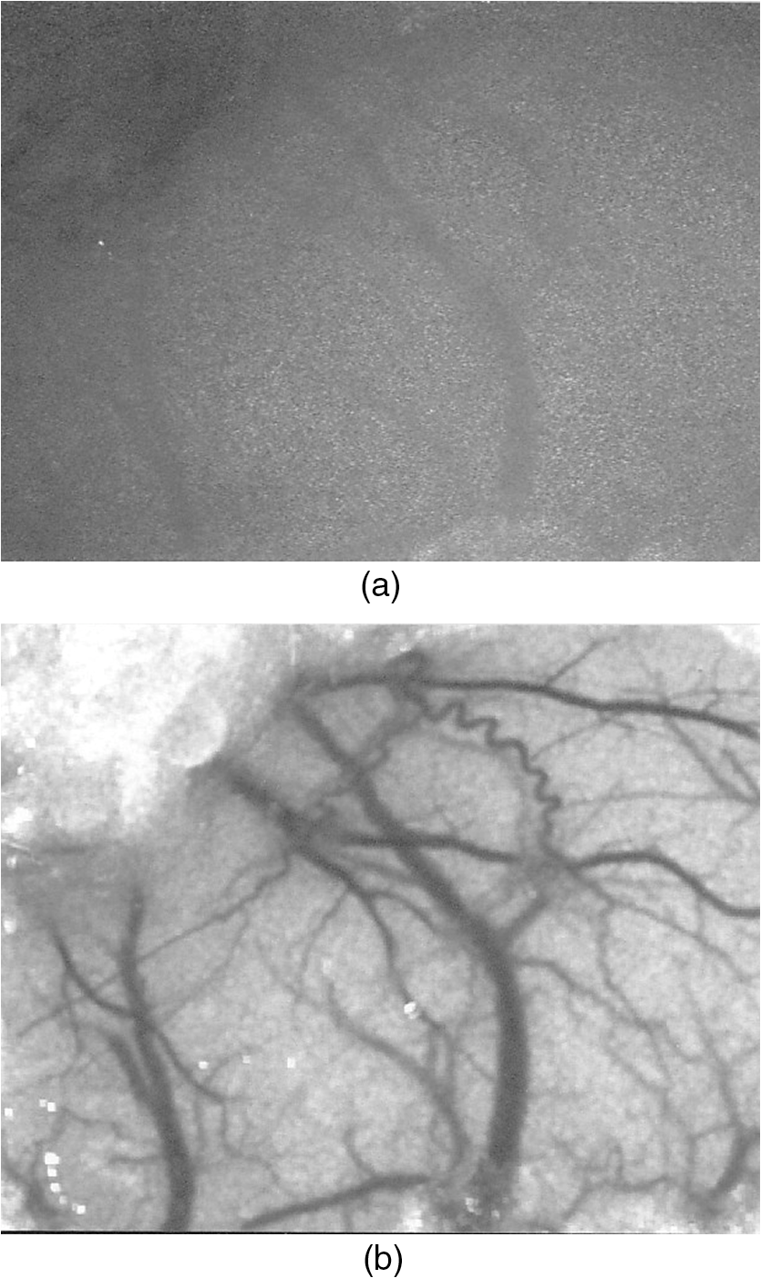
2.1.

Laser Speckle

When laser light illuminates a diffuse surface, the high coherence of the light produces a random granular effect known as speckle. Figure 1 shows a typical speckle pattern.

Fig. 1

A typical laser speckle pattern.

Laser speckle is an interference pattern produced by light reflected or scattered from different parts of the illuminated surface. If the surface is rough (surface height variations larger than the wavelength of the laser light used), light from different parts of the surface within a resolution cell (the area just resolved by the optical system imaging the surface) traverses different optical path lengths to reach the image plane. (In the case of an observer looking at a laser-illuminated surface, the resolution cell is the resolution limit of the eye and the image plane is the retina.) The resulting intensity at a given point on the image is determined by the superposition of all waves arriving at that point. If the resultant amplitude is zero because all the individual waves cancel out, a dark speckle is seen at the point; if all the waves arrive at the point in phase, an intensity maximum is observed.

Laser speckle is a random phenomenon and can only be described statistically. Goodman¹ has developed a detailed theory, but for this paper only one result is of major importance. This is an expression for the contrast of a speckle pattern. Assuming ideal conditions for producing a speckle pattern—highly coherent, single-frequency laser light; linear polarization; and a perfectly diffusing surface—Goodman showed that the standard deviation of the intensity variations in the speckle pattern is equal to the mean intensity. In practice, speckle patterns often have a standard deviation that is less than the mean intensity and this causes a reduction in the contrast of the speckle pattern. In fact, it is normal to define the speckle contrast as the ratio of the standard deviation to the mean intensity:

Although a detailed account of laser speckle statistics is outside the scope of this paper, it is worth mentioning at this point that the scale of the speckle pattern—the size of the individual speckles—has, in general, nothing to do with the structure of the surface producing it. It is determined entirely by the wavelength of the light and the aperture of the optical system used to observe the speckle pattern. If the speckle pattern is being observed directly by the human eye, it is the pupil of the eye that determines the speckle size. More importantly, if a camera is used, it is the setting of the aperture stop that determines the speckle size. This can have a serious effect if the aperture is used to control the exposure of the image.

2.2.

Time-Varying Speckle

When an object moves, the speckle pattern it produces changes. For small movements of a solid object, the speckle pattern moves as a whole, i.e., the speckles remain correlated. For larger motions, the speckles “decorrelate” and the speckle pattern changes completely. Decorrelation also occurs when the light is scattered from a large number of individual moving scatterers, such as particles in a fluid. An individual speckle appears to “twinkle” like a star. This phenomenon has come to be known as “time-varying speckle.” One of the most important potential applications of speckle fluctuations, first recognized by Stern,² arises when they are caused by the flow of blood.

It is reasonable to assume⁵ that the frequency spectrum of the fluctuations should be dependent on the velocity of the motion. It should therefore be possible to obtain information about the motion of the scatterers from a study of the temporal statistics of the speckle fluctuations. This is the basis of the study of time-varying speckle, many of whose applications have been in the biomedical field.

2.3.

Relationship with Laser Doppler

Movement, especially of individual scatterers, causes laser speckle patterns to fluctuate in time. However, laser Doppler techniques also analyze the frequency spectrum of light intensity fluctuations observed when laser light is scattered from moving particles. Are these the same fluctuations? The physics at first sight looks different in the two cases. In the Doppler method, the frequency of light scattered from moving particles is assumed to be frequency-shifted and this “beats” with nonshifted light from stationary parts of the object (or from a reference beam) to give a Doppler signal whose frequency is equal to the difference between the two frequencies. On the other hand, no frequency shift is invoked to explain time-varying speckle—the speckle pattern is produced by interference of light of the same frequency that has traversed different optical path lengths to reach the detector, and the fluctuations are caused by these path lengths changing as a result of the motion of the scatterers. However, the two techniques yield the same mathematical formula connecting the frequency of the fluctuations and the velocity of the scatterers⁶—they are simply two different ways of looking at the same phenomenon.

Whether regarded as Doppler or as time-varying speckle, it is important to note that measurements of the temporal statistics of the intensity fluctuations can, in principle, be carried out only at a single point (strictly, a single speckle). If a map of the velocity is required, some method of scanning is necessary. This has been done for both speckle^7–10 and for Doppler.^11–13 The main problem with these scanning instruments is the time taken for a scan to be carried out and for the data to be processed—typically several minutes. It was for this reason that the technique of LSCI, which produces a map of velocity in a single shot, was developed.

Some workers claim that the main difference between LSCI and laser Doppler is that the former is qualitative and the latter quantitative. In other words, LSCI needs to be calibrated and Doppler does not. We believe there is some confusion here and this needs to be addressed.

It is true that the Doppler technique, as originally envisaged, gives absolute measurements of velocity, but only in a small and well-defined volume, typically $0.1{\mathrm{mm}}^3$ or less, that is defined by two or more laser beams crossing at an oblique angle. These systems are capable of providing, without calibration, absolute velocities in one or more dimensions (depending on the number of laser beams used). One of the beams is typically frequency-shifted, which allows the direction of the movement to be determined and hence the full velocity vector to be measured.

Note that in this paper we are following the current practice of referring to “velocity” when we really mean just its magnitude; when the direction of travel is also known, we shall refer to the “full velocity vector,” as above. We are also using the clinical term “perfusion” for blood flow: the accepted units for this are typically milliliters per 100 grams per minute, or sometimes milliliters per 100 milliliters per minute. This clearly involves concentration and contrasts with other types of flow, where the units for “rate of flow” are volume per unit time. In this paper, we shall use “flow” to mean “rate of flow” and “perfusion” when we are talking specifically about blood flow. It is important, however, to remember the above differences in definition and units.

In contrast to the technique described earlier in this section, the Doppler systems used for perfusion measurements are “regional” rather than point-wise. They still rely on the Doppler shift, but in this case multiple scattering in static structures surrounding the blood vessels will blur the relationship between the direction of the blood flow and the scattering vector. This is further pronounced in tissue, where blood flows in a variety of directions. As a result, a single blood flow velocity will give rise to a distribution of Doppler frequencies that depends not only on the blood flow velocity and concentration but also on the scattering phase function of the red blood cells and the degree of multiple Doppler shifts.

A measure of motion is derived by calculating the first-order moment of this Doppler spectrum, but such measurements provide only relative estimates of regional perfusion (not absolute measurements, as with point-wise systems). These regional measurements are of value when the objective is to measure relative changes in perfusion, for example, due to some stimulus. Quantitative assessment of volumetric flow with these systems is very error-prone and certainly requires calibration.

Note that the above discussion applies equally to both regional laser Doppler systems (such as those used for perfusion measurements) and LSCI. In their original forms, neither can produce absolute measurements of velocity and both require calibration. Fredriksson et al. have recently proposed a tissue and light transport modeling approach aimed at absolute perfusion estimation.¹⁴

We should mention at this point that there are other techniques for imaging blood flow, including spectroscopic methods such as tissue viability and hyperspectral imaging. Our intention in this paper is not to compare LSCI with these other techniques, and we would refer the reader to other publications for such comparisons.^15,16

3.1.

Single-Exposure Speckle Photography

In the early 1980s, Fercher and Briers³ introduced the idea of using speckle contrast reduction to measure flow. They called the technique “single-exposure speckle photography,” in order to distinguish it from the double-exposure method widely used to measure simple movements.

The basic argument is that in a photograph taken under laser illumination, the speckle pattern in an area where flow is occurring is blurred to an extent that depends on the velocity of flow and on the exposure time of the photograph. The speckle pattern in an area of no flow, on the other hand, remains of high contrast. Thus velocity distributions are mapped as variations in speckle contrast.

In practice, contrast variations are difficult for the human eye to detect and some method of enhancing the contrast maps is necessary. Digital techniques were not sufficiently developed in the early 1980s for this to be done as the photograph was taken (though they could have been used on the resulting photograph). Fercher and Briers found, however, that a simple optical filtering process, using a high-pass spatial filter, worked quite well and resulted in the contrast variations being converted into intensity variations. They successfully applied the technique to the mapping of retinal blood flow.¹⁷ Figure 2 shows an example from their 1982 paper.

Fig. 2

Single-exposure speckle photography¹⁷—raw image of part of a retina (a) and its spatially filtered version, showing contrast variations mapped as intensity variations (b).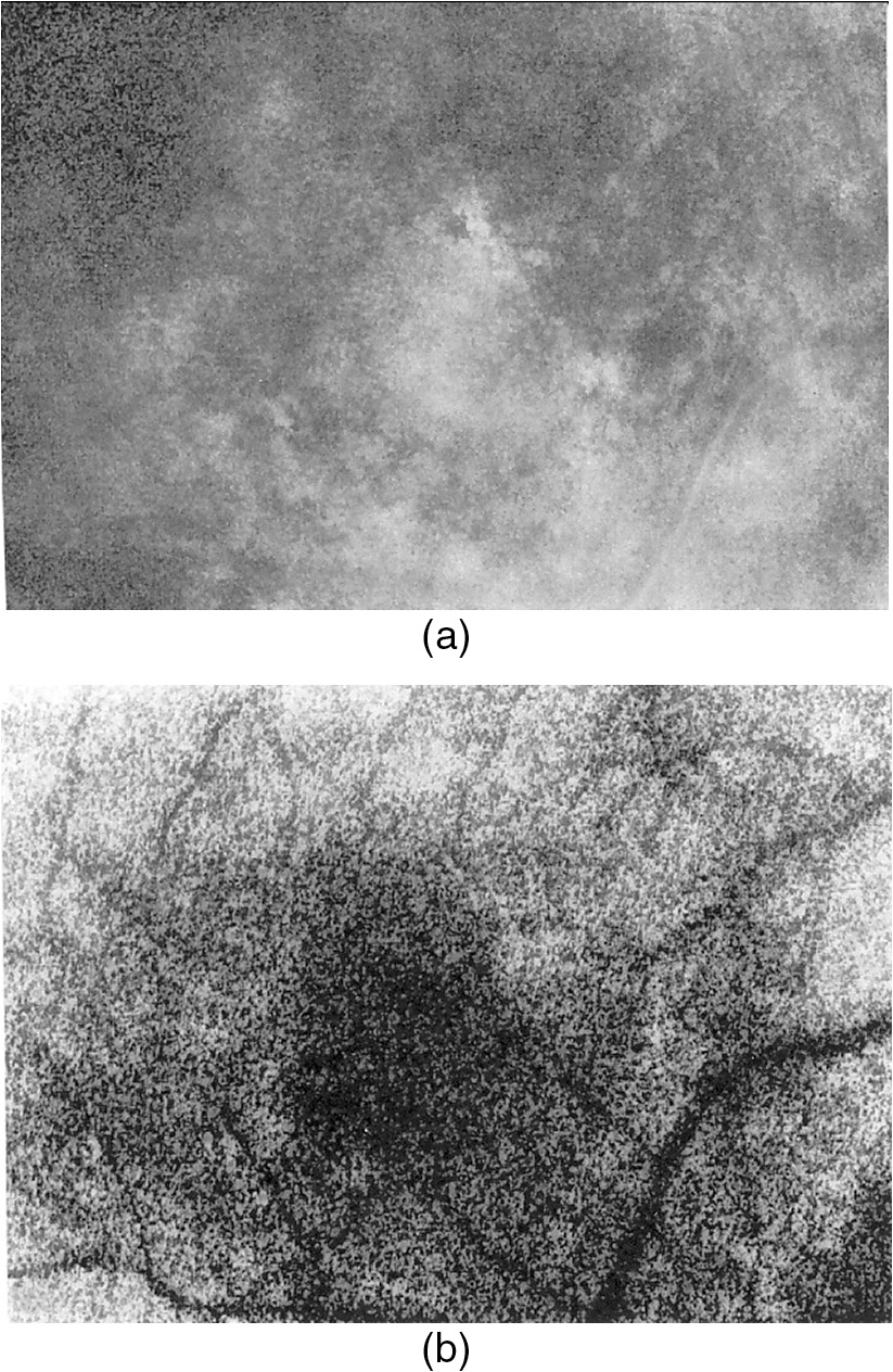

Although the feasibility of single-exposure speckle photography had been demonstrated, the fact that it was a two-step process—the photograph had first to be processed, the resulting transparency had to be placed in the spatial filtering setup, and then a second photograph had to be taken—reduced its attractiveness to clinicians and researchers.

3.2.

Laser Speckle Contrast Imaging: a Digital Version of Single-Exposure Speckle Photography

By 1990, digital techniques were sufficiently advanced to justify taking another look at single-exposure speckle photography. Briers and Webster⁴ succeeded in measuring the contrast directly and converting it to a false-color image, thus avoiding the main disadvantage of the photographic process. As the procedure no longer involved photography, a new name was needed, and they suggested LASCA. Today, alternative names include LSCI and LSI. Figure 3 shows an early example of the original LASCA technique.⁴

Fig. 3

LASCA images of the back of a hand,⁴ showing a change in perfusion caused by rubbing a small area: blue indicates high contrast and therefore little or no flow, while red indicates low contrast and therefore high flow.

3.3.

Some Recent Work on Laser Speckle Contrast Imaging

Several of the authors of this paper—and many others around the world—have developed and improved the techniques of LSCI over the past two decades. Examples include optimization of the exposure time by Boas’s group,¹⁸ a noise reduction scheme by Scheffold’s group,¹⁹ and some significant contributions to the theory.^20–22

Applications have been mainly in the medical field, as expected, with a lot of activity in using the technique to monitor cerebral blood flow.^23–28 Boas’s group has been particularly active in this area and has also used the technique in an investigation into migraines.²⁹ Other medical applications have included microcirculation investigations,^30–32 dentistry,³³ wound and burn assessment,^34–36 and a return to ophthalmological problems.^37–40 Nonmedical applications have included measuring the velocity of vehicles^41,42 and monitoring the drying of paint.⁴³

In addition to the above (and much other) work, there have been several reviews of speckle contrast imaging,^44–48 including some comparative studies with laser Doppler techniques.^49–51

This recent work on LSCI has, of course, been accompanied by improvements in the images produced. Figures 4 and 5 are just two examples—the improvement in the quality of the images is clear (see Figs. 2 and 3).

Fig. 4

Raw image of part of a rat cortex (a) and its LSCI version (b).

Fig. 5

LSCI images of part of a human retina, single exposure above and average of eight successive exposures below.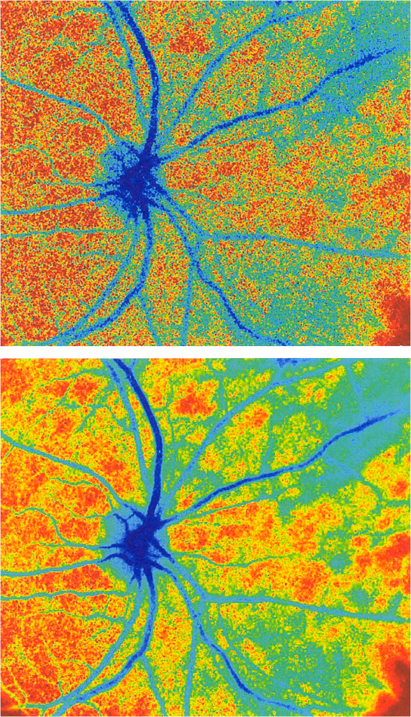

In recent years, at least two companies have launched instruments based on LSCI, both with real-time video capability. These allow the operator to follow changes of flow (in particular, blood perfusion) in real time.

6.1.

Velocity Distribution

Equation (2) shows the relationship between the normalized variance of a time-integrated fluctuating speckle pattern (speckle contrast) and the temporal statistics of the fluctuations (autocovariance). LSCI measures the quantity on the left-hand side of this equation. Laser Doppler, on the other hand, directly measures the temporal statistics of the fluctuations (provided the concentration of moving scatterers is not too large), effectively measuring $C_t^{(2)}(\tau )$ in the right-hand side of the equation. For tissues containing a low concentration of red blood cells, it is widely accepted that the first moment of the Doppler spectrum (the power spectrum of the fluctuations) scales linearly with velocity and concentration.⁵ This means that the regional Doppler techniques used for blood perfusion measurements (see Sec. 2.3) measure changes in the tissue perfusion. In the case of single-exposure LSCI, however, the link between the spatial statistics (speckle contrast) and tissue perfusion can only be made if the velocity distribution is known. In general, this will not be the case. Equation (3), linking speckle contrast with velocity, has been derived by assuming a particular form for the velocity distribution. It is clear from Fig. 6 and the discussion of it above that the choice of velocity distribution has a major effect on this relationship.

The original work on single-exposure speckle interferometry³ and LASCA⁴ assumed a Lorentzian distribution. This is probably appropriate for Brownian motion (unordered flow), but for ordered flow, a Gaussian distribution is usually considered more appropriate. As Duncan and Kirkpatrick have pointed out, there is an argument that the actual distribution is some combination of the two.⁵² It is clear from Fig. 6 that a measurement using a single integration time (and hence a single value of ${\tau }_c/T$) cannot determine which velocity distribution curve is the correct one to use. The question remains as to whether the actual velocity distribution can be determined by other methods and then used to quantify LSCI measurements.

A related issue arises from the fact that LSCI computes the speckle contrast at each point by using the local standard deviation and local mean intensity. This has its own probability distribution, which Duncan and Kirkpatrick have shown to be log-normal.⁵⁶ The result of this is that any velocity estimate derived on the basis of computed local speckle contrast will be a sample statistic with its own attendant probability distribution.

Strictly speaking, the speckle contrast as measured by LSCI is dependent on the correlation time, ${\tau }_c$, and it is usually accepted that this is inversely proportional to some “typical” velocity. However, the constant of proportionality is open to question and depends to some extent on the direction of motion of the scatterers. This will clearly have some impact on the ability of LSCI to measure absolute velocities, flow, or perfusion. A related question is whether non-Newtonian flow (which blood perfusion certainly is) could be an issue.

6.2.

Velocity or Flow?

Equation (3) relates speckle contrast to the correlation time ${\tau }_{c,}$, which is inversely proportional to velocity. It is widely accepted, however, that laser Doppler measures flow (perfusion in the case of blood flow). The question arises: does LSCI measure velocity or flow?

It is easy to show that the speckle contrast must be affected by the number of moving scatterers involved, and hence by the concentration, as this affects the fraction of Doppler-shifted photons. A speckle pattern produced only by stationary scatterers under ideal conditions, will have a speckle contrast of 1 (the maximum). If just a few moving particles are added, it is clear that some intensity fluctuations will be introduced, so that a time-integrated image of the speckle pattern will show some loss of contrast. However, the intensity of each individual speckle will show only small fluctuations about its original (stationary) value. This means that the speckle pattern will be dominated by the pattern from the stationary scatterers and the loss of contrast will be small, even for long integration times. As the number of moving scatterers is increased, the effect of the stationary scatterers will diminish and, for a given integration time, the speckle contrast will decrease. The effect on the graph of speckle contrast against ${\tau }_c/T$ is illustrated schematically in Fig. 7. It is clear that a measurement using a single integration time (and hence a single value of ${\tau }_c/T$) cannot determine whether the continuous or the broken (or any other) curve is the correct one to use.

Fig. 7

Theoretical speckle contrast as a function of the ratio of the speckle correlation time to exposure time, for a completely dynamic medium (solid line) and a medium with a fraction of stationary scatterers (broken line) (schematic only).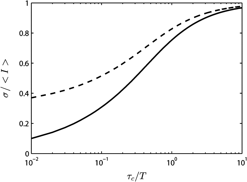

In 1978, Briers⁵⁷ presented a theoretical analysis of the speckle contrast produced by a mixture of moving and stationary scatterers over a long integration time and deduced the following simple relationship between $K$, the speckle contrast, and $\rho$, the fraction of photons in the scattered light that are Doppler-shifted:

In 2003, Rabal et al.⁵⁸ confirmed this equation experimentally. In theory, Eq. (4) could be used on a long-exposure LSCI image to fix the minimum-contrast point on the broken curve of Fig. 7, a contrast value that is strongly dependent on the concentration of moving scatterers rather than their velocity. However, it should be noted that the presence of a static component may also change the shape of the curve.^59,60 From Figs. 6 and 7, it is clear that single-exposure LSCI cannot be related to perfusion in the same way as laser Doppler, without knowledge or assumptions regarding the velocity distribution and the fraction of photons that are Doppler-shifted.

6.3.

Multiple Scattering

It is usually assumed that the photons detected in LSCI have been scattered only once from a moving blood cell. However, it is becoming increasingly clear that some multiple scattering will occur. In tissues with high blood volume fractions, such as the brain, even if light scatters within a vessel no more than once, there is a high probability of detected photons scattering from more than one blood cell from different vessels. One effect of this will be that the technique will be sensitive to the relative motion of blood cells as well as to their absolute motion. As discussed in Sec. 2.3, multiple scattering also means that even a single blood flow velocity will give rise to a distribution of Doppler frequencies, i.e., a spectrum. This leads to the need for both LSCI and Doppler systems, when used to monitor perfusion, to be calibrated.

6.4.

Speckle Size and Polarization

In Eq. (3), the factor $\beta$ is intended to account for the loss of correlation related to the ratio of the detector size to the speckle size, and to polarization.⁵⁵ However, it is not clear whether the invoking of this factor can accurately and reliably compensate for these problems. Kirkpatrick et al.⁶¹ have carried out a detailed investigation of the effect of speckle size on speckle contrast. Thompson et al.²² have shown that a linear $\beta$ correction is valid for simple phantoms and this result may be generalizable to tissue measurements.

7.1.

Velocity Distribution

In order to make the link between the spatial statistics of single-exposure time-integrated speckle patterns (used in LSCI) and the temporal statistics of the intensity fluctuations (used in laser Doppler), it is necessary to know, or assume, the form of the velocity distribution. Poor assumptions are, however, likely to introduce significant errors. It is possible, though, that initial experiments on the type of target to be used might lead to an improved approximation for the distribution, which could then be used in Eq. (3). In 2008, Duncan and Kirkpatrick⁵² suggested a more physically realistic description of the velocity distribution, based on the normalized intensity covariance as expressed by Goodman¹. This “rigid-body” model is an intermediate between the limiting Lorentzian and Gaussian solutions and closely resembles the Lorentzian expectations for long exposures (relative to the correlation time) and the Gaussian expectations for short exposures.

The alternative is to measure the velocity distribution. Thompson and Andrews⁶² have suggested that this can effectively be done by using multiple exposures. They showed that between 10 and 15 exposures, with each successive exposure being double the previous one, are sufficient to produce data on a par with Doppler techniques. The question that arises is whether this can be done while maintaining the real-time advantage of LSCI.

7.2.

Velocity or Flow?

For laser Doppler methods, there is a generally accepted link between the first-order moment of the power spectrum and flow (perfusion in the case of blood).⁵ There is no such accepted theory in the case of laser speckle contrast techniques. Figure 7 shows qualitatively that the presence of stationary (or very slow-moving) scatterers in the field affects the measured speckle contrast. Hence, flow, which depends on the fraction of moving scatterers (e.g., blood in tissue), must have an effect. Whether the technique measures flow, or some quantity related to flow, is an open question and merits further work. Some work has been done on how the presence of static background speckle (e.g., from nonmoving tissue) affects LSCI measurements and some success has been achieved, notably by Zakharov et al.⁵⁹ and by Parthasarathy et al.⁶³ Another possibility might be to combine LSCI with other concepts, such as structured illumination, as suggested by Cuccia et al.⁶⁴

Some initial work by Draijer et al.⁶⁵ has shown that using the parameter $1-K^2$ rather than $K$ has some advantages, in that it can be shown to be a frequency-weighted integral of the power spectrum. In fact, as the integration time $T$ goes to infinity, the quantity $1-K^2\to M_0$, the zero-order moment of the power spectrum, and hence depends strongly on the concentration of moving particles. This to some extent quantifies Fig. 7, as $T\to \infty$ implies ${\tau }_c/T\to 0$. It is worth investigating whether $1-K^2$ gives a better agreement with laser Doppler measurements. However, with the inclusion of non-Doppler-shifted photons, Eq. (3) needs to be revised.

7.3.

Correlation Time and Velocity

Further work is needed on the actual relationship between correlation time ${\tau }_c$ and velocity. Formulae in the literature vary by factors of up to 30 or more, depending on the assumptions made (especially on the effect of multiple scattering). Simple dimensional arguments require that velocity and correlation time be related through a spatial scale length. This is usually taken to be the wavelength of the light, but it is the dimensionless multiplying constant that causes the problems. Perhaps we can avoid the problems if we can relate the speckle measurements to flow rather than velocity.

7.4.

Multiple Doppler Scattering

There is no doubt that multiple Doppler scattering is highly likely to occur and may be difficult to quantify. The degree of multiple scattering will depend on the circumstances of the field being monitored and may well be different for each measurement made. A theoretical solution to this problem may well be insoluble, although Monte Carlo techniques may go some way toward this.

There is also a potentially very significant issue in the presence of multiple populations of scatterers with different correlation times (and hence velocities), all within the same depth of field. The scattered light from the different populations will combine to give a time-varying speckle pattern with a decorrelation behavior somewhere between those of the two (or more) populations independently. It is possible that blind deconvolution techniques may find a solution, but the lack of a priori information about multiple populations will make this very difficult, and perhaps also insoluble. Note that both these problems may also affect laser Doppler measurements.

7.5.

Speckle Size and Polarization

Both these factors will affect the absolute interpretation of the speckle contrast in terms of flow or velocity, but it is less clear whether or not they will affect relative measurements. Hence, although further work is needed on their impact, it is possible that they will not affect measurements of changes in flow (or perfusion in the case of blood), or of variations in flow across an image.

8.1.

Calibration

Although there is no doubt that LSCI is a powerful technique for mapping blood perfusion (and other flow fields) in real time, the physics of the scattering process is so complex and indeterminate that we believe it might never be possible to make absolute measurements. Work will no doubt continue on trying to find solutions to the problems, but in the meantime our recommendation is to regard LSCI as a semi-quantitative technique that requires calibration. (Note that the discussion in Sec. 2.3 indicates that regional Doppler techniques, such as those used in perfusion measurement systems, also require calibration.)

Users of the technique (including the manufacturers of commercial instruments) tend to use a calibration on a phantom to fix a point on a scale and all measurements are made relative to this in arbitrary “perfusion units.” The speckle contrast values are not converted to absolute values of flow, nor are they linear relative to absolute flow.

Because of the uncertainty surrounding the actual velocity distribution that should be used, one approach is to use a much simpler, arbitrary function that produces an S-shaped curve similar to that of Fig. 6. This is done in order to simplify the algorithm and speed up the processing. Possible candidates include the functions $1/K-1$ and $1/K^2-1$ (or their square roots). It can be seen that both these functions go to zero as $K$ approaches 1 and go to infinity as $K$ approaches 0, as required. They are, of course, arbitrary, but the argument is that any velocity distribution chosen is also arbitrary.

8.2.

Multiple Exposures

Thompson and Andrews⁶² have shown that the velocity distribution problem might be solved by using multiple exposures with different integration times. This allows the Doppler spectrum to be computed. If this can be done quickly enough to preserve the real-time operation of LSCI, then it could go a long way toward solving one of the key problems of the technique. It may also answer the velocity/flow argument, though this is not yet clear. Two of the key questions to be answered are the number of exposures required and whether the technique can be made robust against motion artifacts. We believe this approach should be investigated further and that manufacturers should consider incorporating a multiple-exposure option into their instruments.

8.3.

Future

The present situation is that LSCI is a valuable technique for the semi-quantitative real-time mapping of flow fields (including blood perfusion), but that it has to be calibrated and the results are in arbitrary units and not directly related to (or linear with) actual flow values. (Note that the Doppler technique also requires calibration, as discussed in Sec. 2.3.)

The incorporation of multiple exposures will, we believe, improve the quantification of LSCI by effectively allowing the velocity distribution and the fraction of photons that are Doppler-shifted to be measured. The number of exposures needed will have to be investigated.

Further theoretical work, including techniques such as Monte Carlo simulations and blind deconvolution, may improve the robustness of the theory, but not, we think, to the extent that a truly quantitative technique can be achieved.

Because of the complexity of the physical processes and the need (at present) to calibrate LSCI instruments, we recommend that some effort be put into the formulation of a standard experimental configuration for LSCI experiments. (Again, note that the same arguments apply to Doppler techniques.)

In the long term, it is likely that improvements in computer power will allow the parallel processing of laser Doppler images to produce real-time maps. In fact, initial steps to realize this have already been made.⁶⁶ We believe, however, that LSCI will still offer some advantages, for example, where the more expensive Doppler techniques would be an overkill or when maximum temporal resolution is required, and that it will continue to be a valuable tool for the real-time mapping of blood perfusion and other flow fields.