2.1.

Biochemistry of Bone and Overlying Soft Tissues

Bone is a composite of inorganic mineral and organic matrix components. The inorganic component is made up of calcium and phosphate and is often characterized as a carbonated, poorly crystalline hydroxyapatite. The organic matrix of bone is composed of approximately 90% type I collagen by dry weight.⁴⁰ The biomechanical properties of bone and its susceptibility to fracture in both health and diseases is affected by changes to these components and is not limited to BMD. Bone can be classified into two types, cortical bone and trabecular bone, on the basis of porosity and microstructure. The long bones, such as the tibia, have an outer shell of dense cortical bone with the proximal and distal ends, in the regions known as the epiphyses and metaphyses, reinforced internally by a more porous, mesh-like trabecular bone.

The primary soft tissues that contribute interfering signals to transcutaneous Raman measurements include dermal tissue, adipose tissue, and muscle. Transcutaneous Raman spectroscopy is particularly challenging since type I collagen is abundant both in the organic matrix of bone and in soft tissue (e.g., dermal tissue is composed of approximately 80% type I collagen by dry weight⁴⁰). Although it exhibits a unique pattern of covalent cross-linking in bone,⁴¹ type I collagen is genetically identical in all tissues,⁴² so determining the amount to assign to each tissue region is difficult. Representative Raman spectra of murine bone and soft tissue are displayed in Fig. 1.

Fig. 1

(a) Representative Raman spectrum of bone. Major Raman bands are labeled along with their peak positions (in parentheses) in Raman shift. Bands associated with mineral content are labeled in dark blue and bands associated with the organic matrix are labeled in light blue. Note that ${\mathrm{CH}}_2$ is present both in the organic matrix of bone as well as in adipose tissue found in the medullary cavity. (b) Representative Raman spectrum of soft tissue. Notice the large degree of spectral overlap with the bands associated with organic bone matrix.

2.2.

Spatially Offset Raman Spectroscopy and Band Target Entropy Minimization

In SORS, Raman scattered light is collected from surface locations that are spatially offset from the illumination location. The spectral contribution from the subsurface layers relative to the contribution from the superficial layer increases with the magnitude of the offset. In the case of transcutaneous Raman spectroscopy of bone, spectra have typically been acquired at multiple spatial offsets. The variation between spectra is then analyzed, often with BTEM, to estimate the spectrum of the underlying bone.

BTEM is an example of a self-modeling curve resolution algorithm; i.e., it uses a set of mixture spectra (in the present case, from SORS data sets) to estimate the spectrum of a single pure component. The spectral estimate is constructed from the principal components of the mixture spectra based on the minimization of an objective function. In the case of transcutaneous measurements of bone, the dominant ${\mathrm{PO}}_4^{3-}$ ${\nu }_1$ peak (the largest peak in Fig. 1) is targeted, and the BTEM process dictates how the principal components are coadded to render a spectrum exhibiting that peak and others. Despite the success of BTEM in other applications, we show in this publication that the assumptions made by the algorithm are insufficient to produce accurate estimates of bone spectra due to the fact that spectrally similar chemical components (e.g., type I collagen) are present in both bone and soft tissue.

4.1.

Instrumentation and Spectral Processing

All soft-tissue, exposed-bone, and transcutaneous-bone spectra were acquired on a locally constructed Raman spectroscopy system that utilized an 830-nm semiconductor laser (Model PI-ECL-830-500-FS, Process Instruments Inc., Salt Lake City, UT) to deliver approximately 150 mW of power to the sample as shown in Fig. 2(a). The laser light was filtered with a bandpass filter (Chroma Technology Corp., Bellows Falls, Vermont) and the illumination numerical aperture was 0.34.

Fig. 2

(a) Raman spectroscopy system for transcutaneous and exposed-bone measurements. Light gray corresponds to the laser illumination path and dark gray corresponds to the Raman scattering collection path. Abbreviations: ST, shutter; L, lens; MMF, multimode fiber; BP, bandpass filter; BS, dichroic beam-splitter; MTS, motorized translation stage; NF, notch filter; FB, fiber bundle; SPEC, spectrograph; HG, holographic grating; CCD, charge-coupled device. (b) Image of the fiber bundle geometry. For the transcutaneous measurements submitted to SOLD, the data were binned together yielding three total spectra per acquisition (one from the center fiber and first annulus, one from the next annulus, and one from the last two annuli) as indicated by the semi-transparent green circle and rings. The circular array of collection fibers is rearranged into a line for delivery to the imaging spectrograph so that the Raman scattered light collected by each fiber can be separately recorded.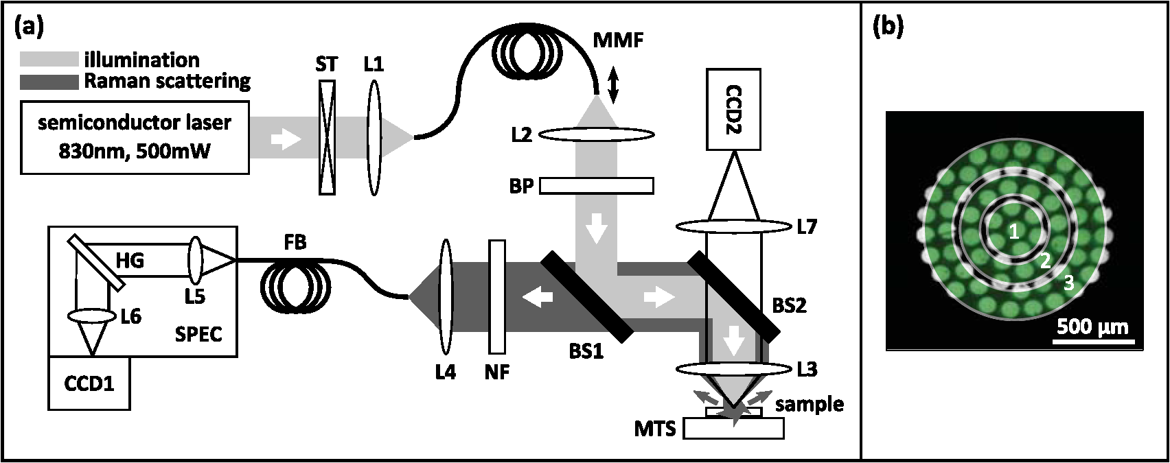

In order to collect the Raman scattered light, lenses L3 and L4 imaged the sample plane onto the face of an optical fiber bundle. The fiber bundle contained 61 multimode optical fibers with $100/120\mu \text{m}$ core/cladding diameters arranged in a circular array at the collection end as shown in Fig. 2(b). The circular array consisted of a center fiber surrounded by four annuli of fibers. For the transcutaneous measurements, the set of spectra acquired by all of the fibers was submitted to BTEM in accordance with the methods used in previous publications. For the transcutaneous measurements submitted to SOLD, the data were binned together yielding three total spectra per acquisition (one from the center fiber and first annulus, one from the next annulus, and one from the last two annuli). For the exposed-bone and soft-tissue measurements, the spectra from all of the fibers were averaged yielding a single spectrum per acquisition.

Each fiber in the fiber bundle viewed a spot of diameter 100 μm at the sample surface. For the transcutaneous measurements, the illumination spot ($1/e^2$ $\text{full}\text{-}\text{width}=230\mu \text{m}$) overlapped with the image of the center fiber of the collection fiber bundle, introducing a range of spatial offsets between the illumination spot and the images of the collection fibers. Although the power delivered by our instrument is greater than the maximum permissible exposure set by the American National Standards Institute,⁴³ no thermal damage was observed. In addition, no adverse consequences were reported in other near-infrared Raman spectroscopy studies of a variety of tissues (including skin) that used power levels greater than ours.⁴⁴ For the exposed-bone and soft-tissue measurements, the illumination spot was defocused ($1/e^2$ $\text{full}\text{-}\text{width}=1000\mu \text{m}$), by adjusting the position of the delivery end of the multimode fiber (MMF in Fig. 2), to overlap with the image of the entire collection fiber bundle. The Appendix contains additional information about the instrument and data processing routines.

After processing, the transcutaneously acquired spectra (and simulated spectra described below) were submitted separately to the SOLD and BTEM algorithms to estimate the spectrum of the underlying bone. The smallest subset of principal components that explained at least 70% of the total variance in each transcutaneous data set was submitted to BTEM, the ${\mathrm{PO}}_4^{3-}$ ${\nu }_1$ peak near $960{\mathrm{cm}}^{-1}$ was targeted, and the spectral estimate was formed by minimizing the objective function suggested by Ong et al.³⁹ The Nelder-Mead downhill simplex method⁴⁵ was used to minimize the BTEM objective function.

4.2.

Simulated Data

Prior to analyzing experimental, transcutaneously acquired data, a simulated data set was constructed to compare the performances of SOLD and BTEM. The parameters described in this section were chosen to generate data sets that resemble transcutaneous spectra acquired from murine tibiae.

4.2.1.

Generation of spectral libraries (L) used to fit simulated data

Spectra of some of the tissue types and chemicals present in bone and soft tissue were acquired as a part of this study. The average spectra of dermal tissue, adipose tissue, and muscle tissue acquired from multiple sites on four different mice are displayed in Fig. 3. Pure ceramic hydroxyapatite (Clarkson Chromatography Products Inc., South Williamsport, PA) was used to represent bone mineral, and dermal tissue was used as a surrogate for the organic matrix of bone since the chemical compositions of these components are similar (approximately 80 and 90% type I collagen, by dry weight, for dermal tissue and organic bone matrix, respectively⁴⁰). The spectral libraries used to generate and fit the simulated data sets were chosen to create an idealized comparison between SOLD and BTEM. More comprehensive libraries were constructed to fit experimental data as described in Sec. 4.3.

Fig. 3

Raman spectra of some of the tissue types and chemical components of bone (blue) and soft tissue (red). Two of the primary components of bone are (a) hydroxyapatite and (b) organic bone matrix. The soft tissues overlying bone include (c) dermal tissue, (d) adipose tissue, and (e) muscle tissue.

4.2.3.

Generation of simulated transcutaneous spectra (M) measured at a single location

The process of simulating the transcutaneous spectra from a single-site measurement is summarized in Fig. 4. The ensemble of SORS spectra was constructed by forming linear combinations of a single pair of bone and soft-tissue spectra [components of a single $\mathbf{S}$ matrix; Fig. 4(a) and 4(b), respectively]. For each source–detector pairing, the bone spectrum was multiplied by a coefficient between 0 and $2/3$ and added to the soft-tissue spectrum. This linear combination was normalized to its mean absolute deviation and added to a spectrum of zero-mean, Gaussian noise [Fig. 4(c)] to form a single transcutaneous spectrum [Fig. 4(d)]. This process was repeated to generate 30 transcutaneous spectra [Fig. 4(e), 4(f), and 4(g)] with varying contributions of the same single pair of bone and soft-tissue spectra. Transcutaneous spectra without added noise were also generated.

Fig. 4

Example of simulated data set used to compare the performances of SOLD and BTEM. The (a) bone and (b) soft-tissue spectra were generated from the spectra in Fig. 3. A spectrum of zero-mean, Gaussian noise (c) was added to a linear combination of the bone and soft-tissue spectra to form a single transcutaneous spectrum (d). This process was repeated to generate 30 transcutaneous spectra [(e), (f), and (g)] with varying contributions of the bone and soft-tissue spectra. These 30 spectra represent a transcutaneous data set acquired from a single measurement site. The set of 30 spectra was submitted to BTEM to estimate the underlying spectrum of bone. In addition, each set of 10 spectra grouped together in (e), in (f), and in (g) was summed, yielding three spectra [(h), (i), and (j)] that were submitted to SOLD. The entire process summarized in this figure was repeated 100 times (with different pairs of underlying bone and soft-tissue spectra) to simulate transcutaneous data acquired from different samples. The gray bars highlight the ${\mathrm{PO}}_4^{3-}$ ${\nu }_1$ peak, which is present in the spectrum of bone. The amplitude of this peak qualitatively represents the contribution of bone to each transcutaneous spectrum.

4.2.4.

BTEM- and SOLD-produced estimates of simulated bone spectrum (one column of S)

The set of 30 transcutaneous spectra was submitted to BTEM to estimate the underlying spectrum of bone. To simulate SORS measurements acquired at three different spatial offsets (corresponding to the three regions depicted in Fig. 2), the 30 transcutaneous spectra were sorted according to the contribution of the underlying bone lineshape. The spectra were then grouped based on their rank order [Fig. 4(e), 4(f), and 4(g)] and each set of spectra was summed yielding three composite spectra [Fig. 4(h), 4(i), and 4(j)] that were submitted to SOLD.

The entire procedure described in Sec. 4.2 to generate and process simulated data is depicted as a flow chart in Fig. 5. This procedure was repeated 100 times (with different pairs of underlying bone and soft-tissue spectra and with or without added noise) to simulate transcutaneous data acquired from different samples.

Fig. 5

Flow chart depicting the procedure used to generate and process simulated data with BTEM and SOLD. This procedure was repeated 100 times (with different pairs of underlying bone and soft-tissue spectra) to simulate transcutaneous data acquired from different samples.

4.3.

Experimental Data

5.1.

Simulated Data

Figure 6 presents the BTEM and SOLD spectral estimates of bone extracted from the single-site, simulated data set shown in Fig. 4. All spectra have been normalized to the height of the ${\mathrm{PO}}_4^{3-}$ ${\nu }_1$ peak near $960{\mathrm{cm}}^{-1}$. Each algorithm was run twice, once upon the simulated data set without added noise [Fig. 6(a) and 6(b)] and once upon the simulated data set with added noise [Fig. 6(c) and 6(d)]. In both cases, SOLD provided a superior estimate of the true underlying bone spectrum [Fig. 6(e)] as evidenced by the accurate reconstruction of the organic bone matrix peaks (e.g., the starred ${\mathrm{CH}}_2$ wag peak near $1450{\mathrm{cm}}^{-1}$). The correlation coefficients between the true and SOLD-estimated bone spectra were both greater than 0.999, while the correlation coefficients between the true and BTEM-estimated bone spectra were 0.985 and 0.968 for the transcutaneous data sets without and with added noise, respectively. All of the spectral correlation coefficients reported in this publication were calculated over the 775 to $1500{\mathrm{cm}}^{-1}$ spectral range, which was chosen to match a previous study.²³ Qualitatively similar results were observed for correlations calculated over a larger spectral range that included the amide I peak near $1665{\mathrm{cm}}^{-1}$.

Fig. 6

Comparison of BTEM and SOLD bone-spectrum estimation methods operating on simulated data. (a) BTEM and (b) SOLD estimates of exposed-bone spectrum from transcutaneous data set without noise. (c) BTEM and (d) SOLD estimates from data set with added noise. (e) True simulated bone spectrum for comparison. To guide comparison, the asterisk highlights the ${\mathrm{CH}}_2$ wag peak, which was more accurately reconstructed with SOLD.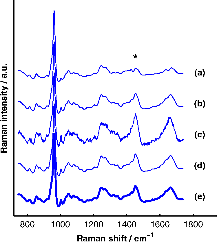

As described previously, the procedure used to generate a simulated, transcutaneous data set was repeated 100 times with a variety of simulated bone and soft-tissue spectra and the transcutaneous data were submitted separately to BTEM and SOLD. The mineral/matrix ratios of all 100 estimated spectra and the corresponding true underlying bone spectra are compared in Fig. 7. The mineral/matrix ratio of each bone spectrum was calculated as the ratio of the fit coefficients produced by least-squares fitting with the pure spectra of hydroxyapatite and organic bone matrix [Fig. 3(a) and 3(b), respectively].

Fig. 7

Scatter plots of estimated versus true mineral/matrix ratios. (a) BTEM and (b) SOLD estimates extracted from simulated transcutaneous data sets without noise. (c) BTEM and (d) SOLD estimates extracted from data sets with added noise. The filled-in markers (highlighted by arrow annotations) correspond to the mineral/matrix ratios of the spectra presented in Fig. 6.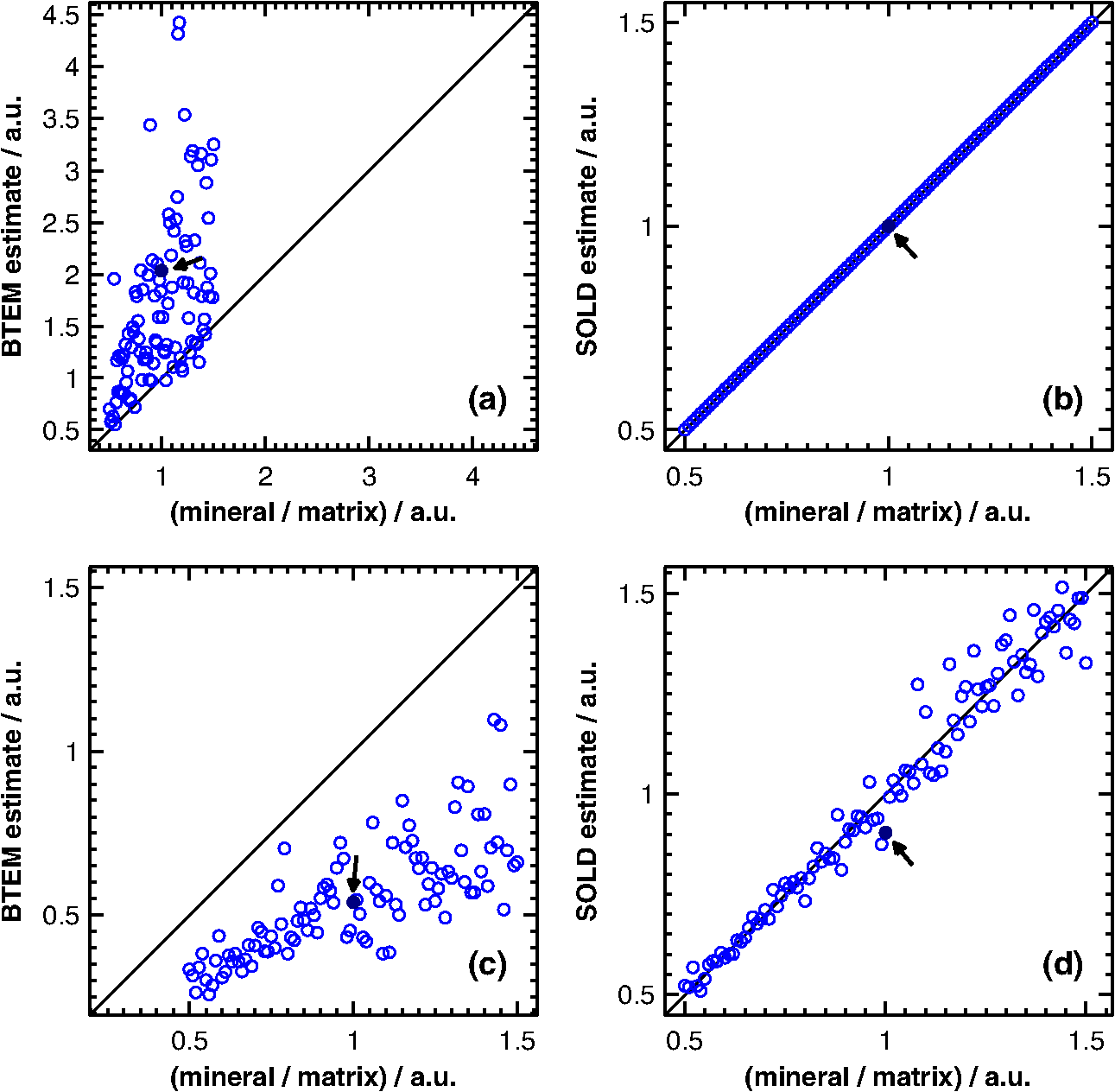

5.2.

Experimental Data

A representative, transcutaneously acquired data set and the corresponding SOLD fit are presented in Fig. 8. As described previously, the transcutaneously acquired spectra were binned together yielding three total spectra per acquisition [Fig. 8(a), green circles] prior to fitting with SOLD. Variation between these spectra is due to differences in the relative sampling of the bone and soft tissue, which is due to different spatial offsets between the illumination spot and the image of each annulus of collection fibers on the surface of the sample [Fig. 2(b)]. All three transcutaneously acquired spectra are well fit by a single bone and a single soft-tissue spectrum [Fig. 8(c) and 8(d), respectively]; as a reminder, these two spectra are formed by linear combinations of the appropriate spectral library ($\mathbf{L}\{k\}$). Spectrum (c) in Fig. 8 is thus the SOLD estimate of the underlying bone spectrum for this particular sample and location on the tibia.

Fig. 8

Representative, transcutaneous spectra acquired at three different source–detector separations (offset for clarity). The measured transcutaneous spectra [(a), green circles] are well fit [(a), black lines] by a single bone (c) and a single-soft tissue (d) spectrum as evidenced by the small amplitudes of the three fit residuals (b).

Figure 9 presents the BTEM and SOLD estimates of the underlying bone spectrum extracted from the data set displayed in Fig. 8. All spectra have been normalized to the height of the ${\mathrm{PO}}_4^{3-}$ ${\nu }_1$ peak near $960{\mathrm{cm}}^{-1}$. Again, SOLD provided a superior estimate of the true underlying bone spectrum [Fig. 9(c)] as evidenced by the accurate reconstruction of the organic bone matrix peaks (e.g., the starred ${\mathrm{CH}}_2$ wag peak near $1450{\mathrm{cm}}^{-1}$). The correlation coefficient between the exposed-bone measurement and the SOLD-estimated bone spectrum was 0.996, whereas the correlation coefficient between the exposed-bone measurement and the BTEM-estimated bone spectrum was 0.935.

Fig. 9

Comparison of BTEM and SOLD bone-spectrum estimation methods operating on experimental data. (a) BTEM and (b) SOLD estimates of exposed-bone spectrum from representative transcutaneously acquired data set presented in Fig. 8. (c) True exposed-bone spectrum for comparison. To guide comparison, the asterisk highlights the ${\mathrm{CH}}_2$ wag peak, which was more accurately reconstructed with SOLD.

The mean correlation coefficients between all of the SOLD-estimated and BTEM-estimated bone spectra and the corresponding gold-standard reference measurements on exposed bone are compared in Table 1. The mean correlation coefficient between the exposed-bone spectra acquired from all of the mice described in Sec. 4.3.1 and the mean correlation coefficient reported in a study by Schulmerich et al.²³ are also tabulated. The Fisher transformation,⁵⁰ along with a Student’s $t$ test, was used to compare the correlations produced by each of the methods. SOLD produced spectra with the greatest correlations to the corresponding reference measurements and the difference between the mean correlation coefficient produced by SOLD and the mean correlation coefficient produced by each other method was statistically significant.

Table 1

Mean correlation coefficients between estimated and/or directly measured bone spectra. The SOLD and BTEM entries refer to correlations between estimated bone spectra and their corresponding reference measurements. The second BTEM entry lists the result reported by Schulmerich et al.23 in the most recent and comprehensive work that can be directly compared to our study. The mean correlation among the spectra of exposed bones from different mice is also listed. Notice that only SOLD produced a mean correlation coefficient greater than this baseline. Statistically significant differences were tested for with unpaired Student’s t tests operating on the Fisher-transformed correlation coefficients. The correlation coefficients produced by each method were compared with those produced by SOLD and in each case the difference was statistically significant.

The SOLD-estimated spectra were also used to predict the mineral/matrix ratios of the corresponding bones. A leave-one-out cross-validation approach utilizing partial least squares regression (PLSR)⁵¹ was used to generate predictions based on the full SOLD-estimated spectra. A scatter plot of these predictions (referred to as PLSR-SOLD) versus the mineral/matrix ratios calculated from the corresponding exposed-bone spectra is displayed in Fig. 10. For the experimental, exposed-bone data sets, the mineral/matrix ratios were calculated as the ratio of the height of the ${\mathrm{PO}}_4^{3-}$ ${\nu }_1$ peak near $960{\mathrm{cm}}^{-1}$ to the heights of the peaks near 855 and $880{\mathrm{cm}}^{-1}$, which are due to vibrations of the amino-acids proline and hydroxyproline, respectively.⁵² All mineral/matrix ratios were normalized to the mean mineral/matrix ratio of the two-month-old WT mice. The relationship between the PLSR-SOLD-derived mineral/matrix ratios and the ratios calculated from the exposed-bone spectra was quantified by a chi-squared test. This test was used to compare the variance of the errors in the PLSR-SOLD estimates (0.030) with the variance of the exposed-bone mineral/matrix ratios (0.176). A one-tailed test revealed that the error variance was significantly less than the variance in the exposed-bone measurements ($p<0.01$), suggesting that SOLD, in conjunction with PLSR, is capable of extracting useful estimates of mineral/matrix ratios.

Fig. 10

Scatter plot of the PLSR-SOLD-estimated mineral/matrix ratios versus the ratios from the corresponding exposed-bone spectra. The filled-in marker (highlighted by the arrow annotation) corresponds to the mineral/matrix ratios of the spectra presented in Fig. 9.

Analysis of the data from the 11 WT mice between 1 and 7 months of age revealed a statistically significant correlation between age and mineral/matrix ratio ($r=0.967$, $p<0.01$). This correlation with age was preserved in the PLSR-SOLD-produced mineral/matrix ratios ($r=0.912$, $p<0.01$). Regarding disease differences, the mineral/matrix ratios of the two-month-old oim/oim mice and WT littermates are compared in Fig. 11. Both the exposed-bone and PLSR-SOLD-derived ratios completely separate the two groups of mice.

Fig. 11

Bar plots of the mean mineral/matrix ratios of WT (white) and $\mathit{oim}/\mathit{oim}$ (gray) mice calculated from exposed-bone spectra and the corresponding PLSR predictions based on the SOLD-estimated spectra. Each circular marker represents the mineral/matrix ratio of a single sample. * $p<0.01$ as determined by a two-sample, unpaired Student’s $t$ test.