|
|
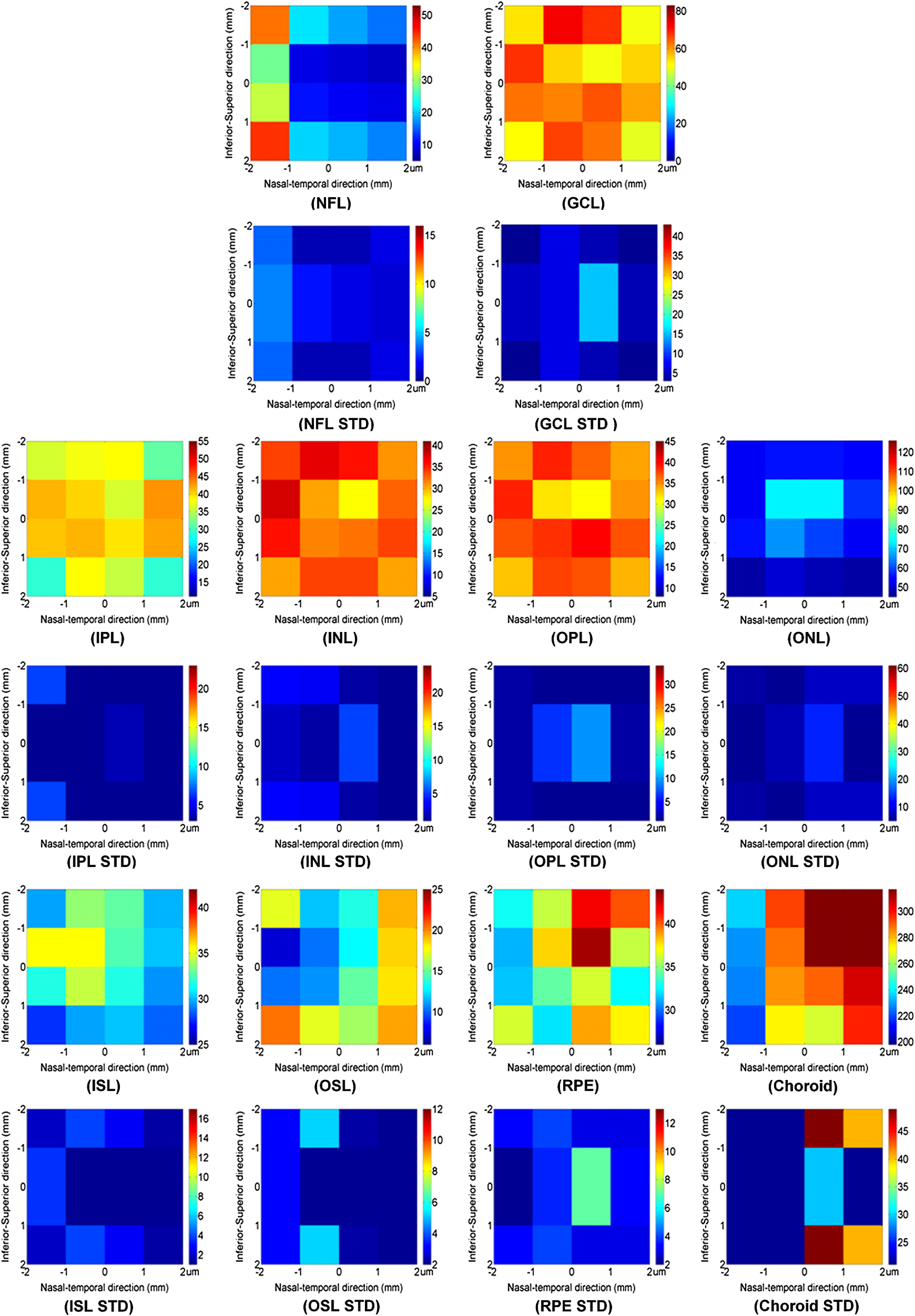
1.IntroductionSpectral-domain optical coherence tomography (SD-OCT) is a three-dimensional (3-D) in vivo imaging technique, which permits direct visualization of retinal morphology and architecture.1 In the setting of retinal or optic nerve disease, the retinal layer thickness may be affected either locally or globally depending on the specific disease; the three most important being age-related macular degeneration (AMD), diabetic retinopathy, and glaucoma.2–4 The identification of the retinal layers and the quantification of their layer-specific properties may facilitate the understanding of the presence and progression of various retinal diseases. Manual tracing of the multiple retinal layers in volumetric SD-OCT images is extremely tedious and time consuming, and thus, automated detection of the multiple retinal layers is attractive. However, the automated detection is not trivial due to the complexity of the layer structures, relatively low-image contrast (especially in the deeper retinal layer bands), and the disturbances produced by various eye diseases. Existing commercial layer segmentation algorithms have largely focused on a few selected inner layers such as the nerve fiber layer (NFL) and ganglion cell layer (GCL). Li et al. developed a graph search framework for the automated multiple layer segmentation of mutually interacting surfaces in 3-D volumetric images.5 This approach was subsequently adapted for multiple retinal layer segmentation in SD-OCT volumes, and has demonstrated a great suitability in several applications.6–10 For instance, Garvin et al. adapted the technique for seven-layer segmentation in retinal SD-OCT volumes.9 Abràmoff et al. applied a fast multiscale scheme to segment four retinal layers.8 However, recent improvements in SD-OCT technology, such as the frame averaging, despeckling techniques, zero delay inversion, and image contrast enhancement, have provided even better definition of the retinal morphology, especially for the deeper posterior segment structures such as the choroidal stroma and choroidal vasculature.11 These high-quality images now provide a broader array of retinal layers that may be the target of segmentation strategies, particularly at the outer aspect of the retina. The outer bands are of particular importance in the pathogenesis and progression of many retinal diseases. Another limitation of most existing layer analysis approaches is an exclusive focus on layer thickness. However, the reflected coherent light carries more potentially valuable information characterizing the optical properties of tissue. The changes in layer intensity/reflectivity may provide further information on the status of the retinal layer in the setting of disease. For instance, our group12 and others13 have recently shown that the reflectivity characteristics may be useful for characterizing and classifying lesions in AMD12 and diabetic retinopathy.13 Thus, as a preliminary investigation, this paper presents an automated graph-based multilayer approach to segment 11 retinal surfaces, including the various retinal bands, in normal SD-OCT images. The intensity/reflectivity and thickness of the various retinal layers were investigated. This investigation in normal subjects may provide a comparative reference for subsequent studies in eyes with diseases. 2.Materials and Methods2.1.MaterialsTwenty eyes of 20 normal subjects with healthy eyes were enrolled in this study at the Doheny Eye Institute of the University of Southern California. The absence of any ocular disease in either eye was confirmed by ophthalmoscopic examination. All subjects provided with written informed consent. The study was approved by the Institutional Review Board of the University of Southern California and adhered to the tenets set forth in the Declaration of Helsinki. For each subject, both eyes underwent volume OCT imaging using a Heidelberg Spectralis (Heidelberg Engineering, Heidelberg, Germany) SD-OCT in accordance with the existing standardized image acquisition protocol utilized by the Doheny Imaging Unit. All volume scans consisted of macular cube scan patterns of () voxels corresponding to the -, -, and -directions, respectively. The physical scan dimensions of each volume varied slightly between cases, but were on average () corresponding to the -, -, and -directions, respectively. The volume scans were obtained with nine frame averaging with the scan oriented for vitreous zero delay. The voxel depth was 8 bits in grayscale. For each subject, one eye was randomly chosen for the subsequent segmentation and analysis. To provide consistency for the quantitative analysis of the retinal layer properties among different volume scans, all the right eyes were horizontally flipped in the -direction. 2.2.Retinal Layer SegmentationOverall, a multistage multisurface graph search segmentation approach5–10 was applied to segment 11 retinal surfaces in the SD-OCT volume scans. The graph search approach used in this study was an evolution of the strategy previously described by Li et al.5 The segmentation of multiple surfaces could be considered as an optimization problem with the goal being to find a set of surfaces with the minimum cost such that the found surface set was feasible. To find a set of surfaces with the minimum cost, a graph with a subset of graphs corresponding to each individual surface was constructed. The cost function was a signed edge-based term, favoring a dark-to-bright or bright-to-dark intensity transition based on different surfaces. It was achieved by applying two different Sobel kernels in the vertical direction convolving with the original SD-OCT image to calculate the vertical derivative approximations. Surface feasibility constraints, i.e., smoothness constraints within a particular surface and interaction constraints between the different surfaces, were applied to limit the neighborhood searching. Thus, the smoothness and the interaction constraints played an important role in accurately segmenting the multiple layers. In Li’s5 previous approach, both the smoothness and the interaction constraints were of a constant value. In our adaptation, the smoothness constraints for both the single surface and double graph search were still constant, which were predefined manually in a similar way as in Ref. 9. However, for the interaction constraints of the double-surface graph searches, the varying constraints with the estimated morphological shape models were employed. More specifically, based on the image intensity features (dark-to-bright and bright-to-dark transition) across the retinal layers, the segmentations of the 11 surfaces were performed in the following sequence: the internal limiting membrane (ILM) and inner—outer segment (IS-OS) junction; outer retinal pigment epithelium (RPE) and choroid-sclera (C-S) junction; inner RPE; the ILM and nerve fiber-ganglion cell (NF-GC) junction; inner plexiform-inner nuclear (IP-IN) and outer plexiform-outer nuclear (OP-ON) junction; GC-IP junction; IN-OP junction; and external limiting membrane (ELM). The detection of the surfaces of the ILM and IS-OS, RPE and C-S, ILM and NF-GC, and the IP-IN and OP-ON junctions used a simultaneous double-surface graph search. The detection of the inner RPE, GC-IP junction, IN-OP junction, and ELM used a single-surface graph search. The ILM was segmented twice for the purpose of helping a better surface detection of the NF-GC junction. To summarize, four simultaneous double-surface graph searches were used to identify seven surfaces, and four single-surface graph searches were used to identify the rest of the four surfaces. For the interaction constraints of the double-surface graph searches, they were still constant for the double surfaces of the ILM and IS-OS junction.9 For the interaction constraints between the ILM and NF-GC junction, based on the observation, in the -direction, the layer thickness in the nasal side has a tendency to be larger and gradually decrease toward the foveal center. In the temporal side, the layer thickness tends to be more constant than that on the nasal side. In designing the interaction constraints for the region of the fovea using the foveal center as a reference, in the nasal side, we applied a mathematical model on the interaction constraints, which had the smallest value at the fovea center and linearly increased along -direction toward the nasal side. In the temporal side, the interaction constraints kept a constant value. In the -direction, the interaction constraints have the same value. In the region outside the fovea, the interaction constraints were also constant. For the double-surface graph search of the IP-IN junction and the OP-ON junction, based on the observation in the region of the fovea, it has the smallest thickness at the foveal center and the thickness gradually increases when moving away from the center. In the design of the interaction constraints, using the foveal center as a reference, a mathematical model was applied on the interaction constraints with the smallest value at the center and linearly increased when moving away from it. In the region outside the fovea, the interaction constraints kept a constant value. For the choroidal band segmentation, based on a recent study from our group14 which evaluated topographical changes in posterior pole choroidal thickness in a cohort of 55 normal eyes, we were able to infer normal, expected regional changes in the choroidal thickness. Specifically, relative to the foveal center, the choroidal thickness shows a significant reduction nasally () and temporally (). In contrast, it shows a slight increase superiorly () and is relatively stable/consistent inferiorly ( decrease). To summarize, the choroidal thickness varies markedly relative to the foveal center in the nasal-temporal direction (-direction in the OCT images) at a range of to , but is relatively stable in the superior-inferior direction (-direction in the OCT images) at a range of to . The normal datasets included in our present study demonstrated a similar regional trend in choroidal thickness. In designing the interaction constraints, in the -direction using the foveal center as a reference, we applied a mathematical model on the interaction constraints, which had the greatest value at the foveal center and linearly decreased bilaterally at each B-scan. In the -direction, the interaction constraints have the same value. To facilitate the multiple surfaces detection, the algorithm performed the segmentation in three different stages by downsampling the raw SD-OCT images in the -direction by a factor of 4, 2, and 1, respectively. Figure 1(a) is an original raw SD-OCT volumetric image. For stage 1 [Fig. 1(b)], the original raw OCT images were downsampled to four times, and the four most detectable and/or distinct surfaces (i.e., ILM, IS-OS junction, outer RPE, and C-S junction) were identified in the four-times-downsampled images using the graph search. The segmented four surfaces were then used as a priori positional information to limit the graph search for the other surfaces at stage 2. In stage 2 [Fig. 1(c)], the original raw OCT images were downsampled to two times, and 11 surfaces were then detected in the two-times-downsampled images using the graph search by incorporating the estimated morphological shape models. In stage 3 [Fig. 1(d)], the segmented 11 surfaces were refined using the same graph search strategy as applied in stage 2, but in the original full resolution image space. Finally, a thin-plate spline fitting15 was applied to smooth the segmented surfaces. The fitting was applied mainly to correct the small localized segmentation errors, most notably in regions of vessel shadows cast by overlying large retinal vessels. Figure 1 illustrates the multistage multilayer segmentation. 2.3.Validation and CharacterizationTo evaluate the accuracy of the automated layer segmentation, the 11 surfaces for each case were manually traced by a certified OCT grader (AH) from the Doheny Image Reading Center, who was masked to the automated results. There was no any refinement by semiautomatic methods before the comparison with manual tracing. Because we desired a high-level of precision, even a single voxel discrepancy in the position of the border at any location was deemed to constitute a discrepancy. The reading center medical director (SS) re-reviewed and confirmed the gradings and boundaries for each case. The accuracy of the automated surface segmentation was evaluated in terms of the mean and absolute mean differences in the -direction between the segmented surfaces and the corresponding manually traced surfaces from the grader. For the mean differences, a negative value indicated that a segmented surface was located above the corresponding manually traced surface, and a positive value indicated that a segmented surface was located below the corresponding manually traced surface. The thickness and intensity/reflectivity properties of the retinal layers defined by the 11 adjacent segmented surfaces were investigated. To provide consistency for the quantitative analysis, the SD-OCT volumetric images were aligned along their foveal centers. For the purpose of the layer thickness analysis, since only the posterior portion of the vitreous was included in volume OCT images, the vitreous was not included in the thickness analysis, and thus resulted in 10 layers of the NFL, GCL, IPL, INL, OPL, ONL, IS, OS, RPE, and choroid layer. The layer reflectivity was normalized against the vitreous and NFL. More specifically, the mean reflectivity of the vitreous was set to zero (i.e., subtracting the mean vitreous intensity from the intensity of the layer of interest), and all the layers were then normalized to the NFL, which had the maximum mean intensity value in the dataset in this study. The vitreous and NFL were specifically chosen because they were consistently the darkest and the brightest layers on the scans. The RPE band is also an intensely bright layer on OCT, but it may be disrupted in various retinal diseases. Thus the NFL was deemed to be a more appropriate choice for normalization for the most retinal diseases of interest. Except for the above 10 layers used in the layer thickness analysis, the visible vitreous was also included in the layer reflectivity analysis. To visualize the thickness and intensity/reflectivity properties in various layers, the mean thickness and normalized mean intensity/reflectivity maps in square grids with a physical size of for each grid subfield were created. Because the SD-OCT volumes used in this study had an unsymmetrical size (average size of ), to better illustrate the grids, we truncated them to a symmetrical size of . 3.ResultsTwenty normal eyes of 20 healthy subjects were included in this analysis. The mean age of the subjects was years (range: 20 to 40 years). Twelve were female and eight were male. Table 1 shows the mean and absolute average border position differences of the 11 surfaces from the ILM to the choroid-sclera junction from the automated segmentation and the manual delineation. The overall mean thickness from the 10 layers between every two adjacent segmented surfaces excluding the vitreous and the overall normalized mean intensity/reflectivity from the 11 layers between every two adjacent segmented surfaces including the vitreous are presented in Fig. 2. The mean thickness grid maps of the 10 layers are shown in Fig. 3, and the normalized mean intensity/reflectivity grid maps of the nine layers (excluding the vitreous and NFL) are shown in Fig. 4. Table 1Mean and absolute mean border position differences of the automated and manual segmentations.
Note: The negative value of the mean differences indicates a segmented surface was located above the corresponding manual delineation, and a positive value indicates the segmented surface was below the corresponding manual delineation. Fig. 2Mean layer thickness and mean layer intensity normalized to nerve fiber layer (NFL). Upper: mean thickness of the 10 retinal layers excluding the vitreous. Bottom: normalized mean intensity of the 11 retinal layers by setting the mean vitreous intensity to zero and normalizing to NFL layer. 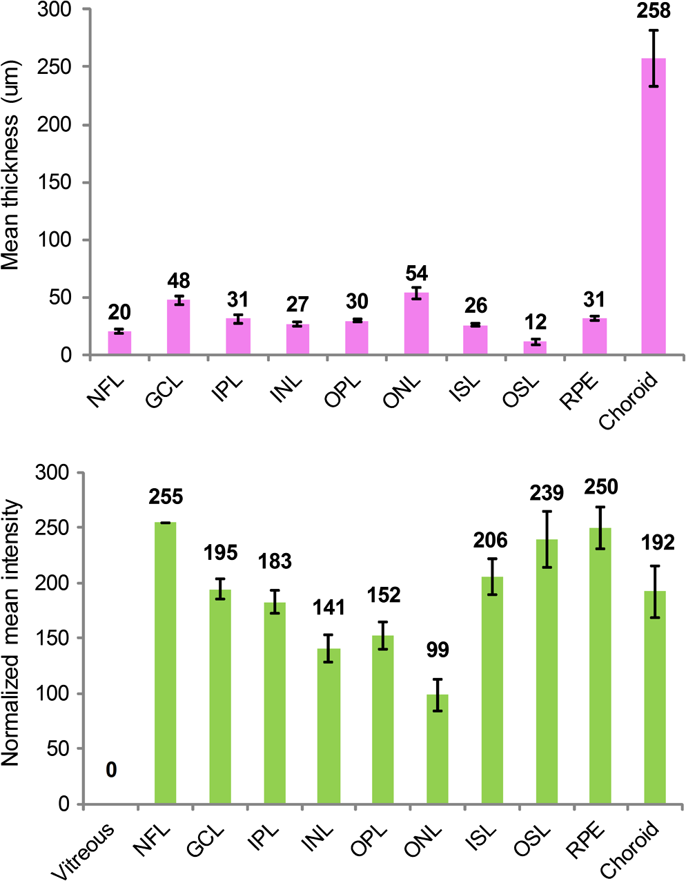 4.Discussion and ConclusionIn this paper, an automated approach was developed to segment 11 retinal surfaces including various retinal bands within the retina on SD-OCT images. The algorithm featured three different stages with various levels of downsampling in order to facilitate the segmentation. The estimated morphological shape models were incorporated to the interaction constraints to constrain the graph search of the retinal surfaces. The overall mean and absolute mean differences in border positions between the automated and manual segmentation for all the 11 segmented surfaces were voxels () and voxels (), respectively, which were both within a subvoxel accuracy, highlighting the robustness of the proposed algorithm for this dataset. While several papers have reported the automated layer segmentation in 3-D SD-OCT images,5–9 to our best knowledge, this is the first study to automatically segment 11 visible retinal layers (now more consistently with current SD-OCT instruments), and is the first to investigate both the thickness and the intensity/reflectivity properties of these layers. The ability to extract these multiple layers provides an opportunity for more in depth analysis of the features and characteristics of the various layers. For example, Figs. 3 and 4 demonstrate the mean thickness and intensity/reflectivity grid maps with a grid subfield. The central coordinate of (0, 0) indicates the foveola location. It is interesting to note that both the mean thickness and normalized mean intensity/reflectivity of the most retinal layers are distributed symmetrically relative to the foveal center. However, for the NFL layer, the mean thickness [Fig. 3(NFL)] is greater nasally compared with that of temporally. For the choroid layer, the mean thickness [Fig. 3(Choroid)] is greater superiorly than inferiorly and is greater temporally than nasally, with the maximum value superiorly and the minimum value nasally. However, for the normalized mean intensity/reflectivity [Fig. 4(Choroid)] of the choroid layer, it is greater nasally than temporally. Changes in both retinal layer thickness2–4 and intensity/reflectivity12,13 may be the indicators of the presence of various eye diseases. Traditionally, the Early Treatment Diabetic Retinopathy Study (ETDRS) grid centered at the foveola was widely used for the analysis of the retinal thickness changes. While an ETDRS grid may be appropriate for neurosensory retinal thickness as a whole, it may not be the optimum choice for layers which are not symmetric relative to the fovea such as the choroid. An ETDRS grid may also not be optimal for presenting regional layer intensity/reflectivity data. The square checkerboard grid presented in Figs. 3 and 4 may be one possible solution. This type of grid may be particularly useful when correlating retinal layer data with functional datasets such as microperimetry-derived retinal sensitivity values. In terms of the speed of the algorithm, the mean segmentation time for all the 11 surfaces was per volume using a Windows 7 workstation with a 2.80 GHz Intel(R) Core(TM) i7 CPU. The segmentation was run on a 64-bit operating system with approximately 8 GB of RAM. In comparison with previous approaches, Garvin et al.10 reported a seven-retinal surface segmentation approach on SD-OCT images, which we believe is comparable with our 11-surface segmentation. The SD-OCT data used in Garvin’s paper was from the Cirrus HD-OCT machines (Carl Zeiss Meditec, Inc., Dublin, California) with an image size of () voxels. As reported, their method was implemented to run on a 64-bit operating system with approximately 10 GB of RAM, requiring hours of processing time per volume to segment all seven surfaces. The images used in this study were obtained from a Spectralis machine with an image size of () voxels. As mentioned above, the total processing time to segment all 11 surfaces was about 4.7 min. Assuming the processing time has a linear relationship with the surface and voxel numbers, we would project that our multistage algorithm would take approximately 6.5 min to process the Cirrus volume scans in Garvin’s study. Thus, we believe the multistage algorithm described in our study has potential to greatly speed up the segmentation of multiple surfaces in OCT volume scans. The algorithm evaluated in this study generally performed well. However, there are several potential targets for further refinement of the technique. For example, structures such as retinal blood vessels may cause optical shadows across the retinal layers, which may confound the detection of surfaces and contribute to layer segmentation errors. This problem, however, could potentially be managed by first identifying the vessel location and performing an interpolation from the surrounding nonvessel region.16–18 We have previously reported a unimodal vessel segmentation approach16 for optic nerve head (ONH) centered SD-OCT images, and a multimodal vessel segmentation approach17,18 for ONH-centered SD-OCT images and color fundus images. Both can be modified for the segmentation of the blood vessels in the macular volumetric scans, and this is a natural target for future studies. In addition, as can be seen from Table 1, the segmentation performance in the outer most bands (inner RPE, outer RPE, and choroid) was worse overall compared with the inner bands. We suspect that this was in part a reflection of the inherent loss of sensitivity with depth at the center wavelength used by the most current commercial SD-OCT devices (870 nm for the Spectralis OCT). The loss of sensitivity would generate increased noise, which would be expected to degrade algorithm performance. This problem may be mitigated by the next generation of swept-source OCT instruments, which feature less sensitivity roll-off and longer wavelengths (e.g., 1050 nm). Our study is not without limitations. First, our study sample was relatively small. Thus, without evaluation in a larger cohort, we cannot be certain that the algorithm will generalize. On the other hand, detailed manual segmentation of 11 surfaces on every B-scan in dense volume OCT scans is exhaustive and difficult to perform for a very large datasets. Second, our sample only included normal eyes. The methods necessary to adapt or tune the algorithm to function in the setting of retinal disease are still uncertain. However, starting with normal is important as it provides an opportunity to collect a normative database of values for future comparison with disease. Third, this pilot study only included normal subjects and with a relatively narrow age range (mean age: years old; 24 to 42 years old). However, the layer thickness may vary with age. For instance, it is known that the choroid thickness decreases with age.19 It is possible that the layer reflectivity may change as well. Fourth, in this study, the foveal center was simply defined as the lowest position of ILM surface. This worked well for this normative data study with horizontally oriented scans. This simple solution may not suffice in the setting of disease or severely tilted scans (e.g., in high myopes), and may require a different solution for foveal detection. Despite these limitations, our study has many strengths as presented above for the automated segmentation, and also including the use of meticulous manual segmentation by expert reading center-certified OCT graders. In summary, we present an automated graph-based multistage multilayer approach integrating the estimated morphological shape models to segment 11 retinal surfaces in normal SD-OCT images. The overall mean and absolute mean differences in border positions between the automated and manual segmentation were both under the subvoxel level, indicating an excellent segmentation accuracy of the proposed algorithm on this dataset. This investigation in normal subjects may provide a comparative reference for subsequent adaptations in eyes with diseases. AcknowledgmentsThis work was supported, in part, by the Beckman Macular Degeneration Research Center and a Research to Prevent Blindness Physician Scientist Award. ReferencesW. DrexlerJ. G. Fujimoto,
“State-of-the-art retinal optical coherence tomography,”
Prog. Retin. Eye Res., 27
(1), 45
–88
(2008). http://dx.doi.org/10.1016/j.preteyeres.2007.07.005 PRTRES 1350-9462 Google Scholar
C. K. Leunget al.,
“Retinal nerve fiber layer imaging with spectral-domain optical coherence tomography: patterns of retinal nerve fiber layer progression,”
Ophthalmology, 119
(9), 1858
–1866
(2012). http://dx.doi.org/10.1016/j.ophtha.2012.03.044 OPANEW 0743-751X Google Scholar
S. E. Chunget al.,
“Choroidal thickness in polypoidal choroidal vasculopathy and exudative age-related macular degeneration,”
Ophthalmology, 118
(5), 840
–845
(2011). http://dx.doi.org/10.1016/j.ophtha.2010.09.012 OPANEW 0743-751X Google Scholar
M. A. Sandberget al.,
“Visual acuity is related to parafoveal retinal thickness in patients with retinitis pigmentosa and macular cysts,”
Invest. Ophthalmol. Vis. Sci., 49
(10), 4568
–4572
(2008). http://dx.doi.org/10.1167/iovs.08-1992 IOVSDA 0146-0404 Google Scholar
K. Liet al.,
“Optimal surface segmentation in volumetric images—a graph-theoretic approach,”
IEEE Trans. Pattern Anal. Mach. Intell., 28
(1), 119
–134
(2006). http://dx.doi.org/10.1109/TPAMI.2006.19 ITPIDJ 0162-8828 Google Scholar
Z. Huet al.,
“Automated segmentation of the optic disc margin in 3-D optical coherence tomography images using a graph-theoretic approach,”
Proc. SPIE, 7262 72620U
(2009). http://dx.doi.org/10.1117/12.811694 PSISDG 0277-786X Google Scholar
Z. Huet al.,
“Automated segmentation of neural canal opening and optic cup in 3-D spectral optical coherence tomography volumes of the optic nerve head,”
Invest. Ophthalmol. Vis. Sci., 51
(11), 5708
–5717
(2010). http://dx.doi.org/10.1167/iovs.09-4838 IOVSDA 0146-0404 Google Scholar
M. D. Abràmoffet al.,
“Automated segmentation of the cup and rim from spectral domain OCT of the optic nerve head,”
Invest. Ophthalmol. Vis. Sci., 50
(12), 5778
–5784
(2009). http://dx.doi.org/10.1167/iovs.09-3790 IOVSDA 0146-0404 Google Scholar
M. K. Garvinet al.,
“Intraretinal layer segmentation of macular optical coherence tomography images using optimal 3-D graph search,”
IEEE Trans. Med. Imag., 27
(10), 1495
–1505
(2008). http://dx.doi.org/10.1109/TMI.2008.923966 ITMID4 0278-0062 Google Scholar
M. K. Garvinet al.,
“Automated 3-D intraretinal layer segmentation of macular spectral-domain optical coherence tomography images,”
IEEE Trans. Med. Imag., 28
(9), 1436
–1447
(2009). http://dx.doi.org/10.1109/TMI.2009.2016958 ITMID4 0278-0062 Google Scholar
B. Sanderet al.,
“Enhanced optical coherence tomography imaging by multiple scan averaging,”
Br. J. Ophthalmol., 89
(2), 207
–212
(2005). http://dx.doi.org/10.1136/bjo.2004.045989 BJOPAL 0007-1161 Google Scholar
S. Leeet al.,
“Automated characterization of pigment epithelial detachment by optical coherence tomography,”
Invest. Ophthalmol. Vis. Sci., 53
(1), 164
–170
(2012). http://dx.doi.org/10.1167/iovs.11-8188 IOVSDA 0146-0404 Google Scholar
W. Gaoet al.,
“Investigation of changes in thickness and reflectivity from layered retinal structures of healthy and diabetic eyes with optical coherence tomography,”
Biomed. Sci. Eng., 4 657
–665
(2011). http://dx.doi.org/10.4236/jbise.2011.410082 1937-6871 Google Scholar
Y. Ouyanget al.,
“Spatial distribution of posterior pole choroidal thickness by spectral domain optical coherence tomography,”
Invest. Ophthalmol. Vis. Sci., 52
(9), 7019
–7026
(2011). http://dx.doi.org/10.1167/iovs.11-8046 Google Scholar
G. DonatoS. Belongie,
“Approximate thin plate spline mappings,”
in Proc. of the 7th Eur. Conf. Computer Vision (ECCV 2002), Part III, Lecture Notes in Computer Science,
21
–31
(2002). Google Scholar
Z. Huet al.,
“Automated segmentation of 3-D spectral OCT retinal blood vessels by neural canal opening false positive suppression,”
in Proc. of Medical Image Computing and Computer-Assisted Intervention (MICCAI 2010), Part III, Lecture Notes in Computer Science,
33
–40
(2010). Google Scholar
Z. Huet al.,
“Automated multimodality concurrent classification for segmenting vessels in 3-D spectral OCT and color fundus images,”
Proc. SPIE, 7962 796204
(2011). http://dx.doi.org/10.1117/12.877880 PSISDG 0277-786X Google Scholar
Z. Hu,
“Multimodal retinal vessel segmentation from spectral-domain optical coherence tomography and fundus photography,”
IEEE Trans. Med. Imag., 31
(10), 1900
–1911
(2012). http://dx.doi.org/10.1109/TMI.2012.2206822 ITMID4 0278-0062 Google Scholar
B. AlamoutiJ. Funk,
“Retinal thickness decreases with age: an OCT study,”
Ophthalmology, 87 899
–901
(2003). OPANEW 0743-751X Google Scholar
|