Computer-aided diagnosis of rheumatoid arthritis with optical tomography, Part 1: feature extraction

Ludguier D. Montejo; Jingfei Jia; Hyun K. Kim; Uwe J. Netz; Sabine Blaschke; Gerhard A. Mueller; Andreas H. Hielscher

doi:10.1117/1.JBO.18.7.076001

15 July 2013 Computer-aided diagnosis of rheumatoid arthritis with optical tomography, Part 1: feature extraction

Ludguier D. Montejo, Jingfei Jia, Hyun K. Kim, Uwe J. Netz, Sabine Blaschke, Gerhard A. Mueller, Andreas H. Hielscher

Author Affiliations +

Journal of Biomedical Optics, Vol. 18, Issue 7, 076001 (July 2013). https://doi.org/10.1117/1.JBO.18.7.076001

Abstract

This is the first part of a two-part paper on the application of computer-aided diagnosis to diffuse optical tomography (DOT). An approach for extracting heuristic features from DOT images and a method for using these features to diagnose rheumatoid arthritis (RA) are presented. Feature extraction is the focus of Part 1, while the utility of five classification algorithms is evaluated in Part 2. The framework is validated on a set of 219 DOT images of proximal interphalangeal (PIP) joints. Overall, 594 features are extracted from the absorption and scattering images of each joint. Three major findings are deduced. First, DOT images of subjects with RA are statistically different (p<0.05 ) from images of subjects without RA for over 90% of the features investigated. Second, DOT images of subjects with RA that do not have detectable effusion, erosion, or synovitis (as determined by MRI and ultrasound) are statistically indistinguishable from DOT images of subjects with RA that do exhibit effusion, erosion, or synovitis. Thus, this subset of subjects may be diagnosed with RA from DOT images while they would go undetected by reviews of MRI or ultrasound images. Third, scattering coefficient images yield better one-dimensional classifiers. A total of three features yield a Youden index greater than 0.8. These findings suggest that DOT may be capable of distinguishing between PIP joints that are healthy and those affected by RA with or without effusion, erosion, or synovitis.

1. Introduction

1.1.

Overview

Over the last decade, the field of diffuse optical tomography (DOT) has progressed from purely theoretical studies and bench-top experiments to clinical trials that explore the utility of DOT in the diagnosis of breast cancer,¹ brain imaging,² and the detection of rheumatoid arthritis (RA).³ While substantial advances have been made in building clinically useful instruments and developing image reconstruction algorithms, much less effort has been spent on developing image analysis tools that can aid in quantifying or detecting the presence of diseased tissue.

In this 2-part paper, we introduce a general approach to computer-aided diagnosis (CAD) for DOT. We apply this approach to images of finger proximal interphalangeal (PIP) joints obtained from 20 healthy volunteers and 33 subjects with RA.³ In Part 1, we establish a framework for extracting features of interest from three-dimensional (3-D) DOT images. The statistical significance of each feature is evaluated with classical statistical methods, including Kruskal–Wallis analysis of variance (ANOVA), Dunn’s test, and receiver–operator-characteristics (ROC) analysis. The intra-class correlation coefficient (ICC) is used to compute the effective sample size (ESS) of our data, which in turn is used to adjust our results for any bias that may be introduced by treating each imaged finger as an independent sample. This step is necessary as we imaged multiple fingers per subject. Through this analysis we establish which individual features are best indicators of RA in terms of diagnostic sensitivity (Se) and specificity (Sp). Links between these best features and physiological processes are identified.

In Part 2, (Ref. 4) we combine multiple individual features from Part 1 to form multidimensional feature vectors. The vectors are used as input to five different classification algorithms: $k$ nearest neighbors ( $k$ -NN), linear discriminate analysis (LDA), quadratic discriminate analysis (QDA), support vector machines (SVM), and self-organizing maps (SOM). Algorithm performance is compared in terms of Se and Sp. For each algorithm we determine the set of features that best differentiates between PIP joints with RA and without RA.

1.2.

Background

The development of CAD tools has been a subject of intense research across many areas of medical imaging and image analysis.⁵^,⁶ Often used to enhance the natural contrast between healthy and diseased tissue, CAD tools have been shown to enhance the diagnostic value of various imaging modalities. Its use in detection and characterization of lesions has been expanded to almost all imaging modalities, including X-ray computed tomography (CT), ultrasound, and magnetic resonance imaging (MRI).⁷^–¹⁰ The medical applications that have seen the most activity in CAD research are X-ray imaging of the breast, chest, colon, brain, liver, and the skeletal and vascular systems.⁷

CAD tools have been particularly successful in enhancing the reading of mammograms. For example, Doi reported that the early detection of breast cancer from mammograms improved by up to 20% when CAD tools were used to aid the diagnostic process.⁷ In another study, LDA and Bayesian Neural Networks (BNN) were employed to investigate the repeatability of CAD based diagnosis of malignant breast lesions with sonography. The best sensitivities and specificities, based on repeatability, were 90% and 66% with BNN, and 74% and 84% with LDA,¹¹ respectively.

Similar results have been obtained with MRI data from breast cancer patients. Backpropagation neural networks have been employed for detection of breast tumors,⁹ artificial neural networks have been used to differentiate between breast MRI images of malignant and benign lesions,¹² and SVM has been used to study the effect of MRI enhancement thresholding on breast cancer detection rates.¹³ Typical sensitivity and specificity values of 73% and 56% have been reported for all cancers.¹⁰

In biomedical optics CAD has been employed only in a very limited number of studies. Two papers related to optical coherence tomography (OCT) explored its utility in the diagnosis of esophageal and cervical cancer.¹⁴^,¹⁵ In another study, logistic regression was used in semi-automatic detection of malignant breast lesions in DOT images,¹⁶ while a fourth study extracts attributes from three imaging parameters obtained by an NIR imaging system and employs an SVM algorithm to distinguish between malignant and benign lesions.¹⁷ A separate effort has focused on the automated detection of contrast-to-noise ratio regions of interest for DOT imaging of breast tissue.¹⁸^,¹⁹ Other studies investigated the ability to discriminate between breast tissue malignancies using tissue fluorescence and reflectance measurements from diffuse reflectance spectroscopy of excised²⁰ and in vivo²¹ breast tissue.

Over the past six years, our group has studied the use of CAD techniques in the field of DOT, with particular emphasis on the diagnosis of RA. Our initial studies involving DOT imaging of arthritic finger PIP joints determined that visual inspection of the reconstructed absorption ( $μ_{a}$ ) and scattering ( $μ_{s}^{'}$ ) coefficient distributions results in low Se and Sp values. The difficulties in diagnosing RA from visual inspection of the DOT images alone motivated the development of CAD tools for use in DOT.

So far, our research on the use of CAD techniques for diagnosing RA has focused on the classification of constant wavelength (CW) DOT images of PIP joints.²² In early work, a small clinical trial was used to obtain data and show that CAD enhanced diagnosis of RA from DOT images might be possible. Basic image features were extracted from $μ_{a}$ images, and linear regression (LR), LDA, and SOM were used for classification. The results were promising, motivating a larger clinical study to more definitively establish the ability to diagnose RA from DOT images. The initial studies were limited in that only CW-DOT scans were performed on PIP joints. As a result, the utility of $μ_{s}^{'}$ images in classification was poor, prompting classification to be performed using only $μ_{a}$ data.²²^,²³

More recently, we reported on the ability to accurately diagnose RA from frequency domain (FD) DOT images of PIP joints using multidimensional LDA.³ In that study we introduced classification of PIP joints using both $μ_{a}$ and $μ_{s}^{'}$ data. The study proved that classification with FD-DOT images (91% Se and 86% Sp) was significantly more accurate than classification with CW-DOT images (64% Se and 55% Sp). Furthermore, the study showed that features derived from $μ_{s}^{'}$ images allowed for more accurate classification (91% Se and 86% Sp) when compared to $μ_{a}$ derived features (83% Se and 83% Sp). A limitation in that study was that classification was not performed using a mixture of $μ_{a}$ and $μ_{s}^{'}$ derived features.

While previous studies employ only basic feature extraction schemes and basic image classification techniques, they do show that there is a significant level of natural contrast in the optical properties of PIP joints, likely arising from the onset of RA. Those results indicate that DOT is a promising technique for diagnosing RA. Results from this 2-part paper further demonstrate the utility of CAD in enhancing our ability to diagnose RA from DOT images.

2. Methods

2.1.

Clinical Study

2.1.1.

Rheumatoid arthritis

The etiology of RA is unknown, however, it is the most common inflammatory arthritis.²⁴ RA is associated with significant pain and disability, affecting about 1% of the world’s population, and approximately 1.3 to 2.1 million people in the US.²⁵ In the US alone, RA leads to 9 million physician visits per year.²⁴ Patients with RA can suffer from severe pain, joint stiffness, swelling of multiple joints, and lack of joint mobility. The joints most often affected by RA are the wrists, metatarsophalangeal, and PIP joints.²⁴ These symptoms can eventually lead to severe disabilities and loss in quality of life.

In practice, the diagnosis of RA is based on the patient’s history, physical exams, radiographs, and laboratory studies. The American College of Rheumatology (ACR) has recommended criteria for the classification of RA (the so-called “ACR 2010 criteria”).²⁶ Early diagnosis of RA is particularly difficult when patients experience nonerosive symptoms (such that they cannot be detected by radiography, sonography, or MRI scans) and in the absence of the rheumatoid factor (RF) and anti-cyclic citrullinated peptide (CCP) antibodies.²⁷

Of all imaging modalities, X-ray imaging has the best-established role in the assessment of the severity of RA.²⁸ Radiography can document bone damage (erosion) that results from RA and visualize the narrowing of cartilage spaces. However, it has long been recognized that radiography is insensitive to the early manifestations of RA, namely effusion and hypertrophy of the synovial membrane. The role of ultrasound and MRI in the detection and diagnosis of RA has been a topic of debate.²⁹ In recent years ultrasound imaging has emerged as a potentially useful technique for diagnosing RA, as it appears to be sensitive to joint effusions and synovial hypertrophy.²⁹ Sensitivities and specificities up to 71.1% and 81.8%, respectively, have been achieved with power Doppler ultrasound,³⁰ while contrast-enhanced MRI has been used to achieve sensitivity and specificity of 100% and 78%, respectively.³¹

In its early stage, RA is characterized by inflammatory synovitis that leads to edema in the synovial membrane (synovium) and joint capsule. The permeability of the synovium is changed, leading to an increase of fluid and large cells in the synovial cavity. These changes are believed to be the source of optical contrast that is observed in DOT images and the motivation for exploring the ability to diagnose RA from DOT images.

Given the current state of treatment and diagnosis, researchers in the field have called for improved early detection of RA so that disease-modifying antirheumatic drug (DMARD) therapies can be initiated earlier as this would significantly help with the management of the disease.²⁴ Additional motivation for establishing DOT as a clinically useful tool for diagnosing RA has to do with patient health and comfort: DOT does not expose subjects to ionizing radiation, contrast agents do not need to be used, and imaging is done contact free. As a result, subjects can undergo routine DOT examinations without the risk of adverse side affects and discomfort.

2.1.2.

Clinical data

We recently reported a clinical study where PIP joints II to IV of 53 volunteers were imaged using a FD-DOT system, including 33 subjects with various stages of RA and 20 healthy control subjects.³ Each subject was evaluated by a rheumatologist and diagnosed for RA according to guidelines set by the ACR.²⁶ The clinically dominant hand of each subject was imaged with ultrasound and low-field MRI.

The ultrasound and MRI images were evaluated by a radiologist and a rheumatologist in a blinded-review. The images were evaluated for the presence of effusion, synovitis, and erosion in PIP joints II to IV. Each reviewer classified each subject into one of five sub-groups on the basis of these findings (Table 1). A third reviewer served as a tiebreaker in cases where the initial reviewers had differing opinions (none in this study). Subjects without signs of joint effusion, synovitis, and erosion were divided into two subgroups: (1) subjects with RA and (2) subjects without RA.

Table 1

Diagnostic table based on clinical evaluation and radiological imaging (ultrasound and MRI).

Group	Effusion	Erosion	Synovitis	RA	Total joints
$A$	No	No	No	Yes	18
$B$	Yes	No	No	Yes	18
$C$	No	Yes	No	Yes	12
$D$	No	No	Yes	Yes	27
$E$	Yes	Yes	Yes	Yes	24
$H$	No	No	No	No	120

Imaging with a FD-DOT sagittal laser scanner of PIP joints II to IV was performed on the clinically dominant hand of subjects with RA and on both hands of the control group. A frequency-modulated laser beam (670 nm, 8 mW, 1.0 mm diameter) scanned the dorsal side of the finger from proximal to distal end, stopping at 11 discrete locations to allow for data acquisition. Transillumination was recorded from each source position on the ventral side of the finger with an intensified CCD camera. The 3-D geometry of the scanned finger was obtained with a separate laser-scanning unit (650 nm, 5 mW, 0.2 mm line width). Imaging was performed at 0, 300, and 600 MHz. In total, 219 fingers were imaged. Transillumination measurements were used to reconstruct tissue $μ_{a}$ and $μ_{s}^{'}$ coefficients with a PDE-constrained optimization algorithm that uses the equation of radiative transfer (ERT) to model propagation of NIR light in tissue. The system and imaging procedures are described in detail by Hielscher et al.³

Each FD-DOT reconstruction results in volumetric distributions of $μ_{a}$ and $μ_{s}^{'}$ within a given finger (Fig. 1). Examples of cross sections are shown in Fig. 2. The most pronounced differences between joints of subjects affected by RA and of subjects not affected by RA occur at the center of the images, the region were the joint cavity is located. As expected, in healthy joints both $μ_{a}$ and $μ_{s}^{'}$ often appear to be lower in this region than in the surrounding tissues. The synovial fluid that fills the joint cavity is almost free of scattering and has a lower optical absorption coefficient than surrounding tissue. Joints affected by RA typically do not show a drop in optical properties in these regions. However, we found that relying on visual inspection of DOT images alone did not yield high sensitivities and specificities. Therefore, we started to explore the use of CAD tools to enhance diagnostic accuracy.³

Fig. 1

Visualization of typical finger geometries. Sample $μ_{s}^{'}$ cross sections are visualized within the finger geometry: (a) coronal ( $x y$ ), (b) sagittal ( $x z$ ), and (c) transverse ( $y z$ ) planes.

Fig. 2

(a and b) Absorption and (c and d) scattering coronal cross sections of PIP joints from subjects without (a, c) and with RA (b, d). All images are reconstructed from the data obtained with 600 MHz source modulation.

2.2.

Data Pre-processing

The reconstructed optical property maps shown in Fig. 2 are originally recovered on a 3-D unstructured mesh with tetrahedral elements. To simplify the data analysis process, we use interpolation to convert the reconstruction data from an unstructured mesh to a structured Cartesian grid. This is a three step process: (1) define a structured grid that overlaps the tetrahedral mesh; (2) identify the set of structured grid points $n_{p}$ whose $x - y - z$ coordinates are within the tetrahedral element defined by the set of four unstructured mesh nodes $p = {r_{1}, r_{2}, r_{3}, r_{4}}$ , where $r_{i}$ refers to the $x - y - z$ coordinates of a node in the unstructured mesh; (3) use interpolation to compute the $μ_{a}$ and $μ_{s}^{'}$ values at structured grid point $k$ ( $\forall k \in n_{p}$ ) using the reconstructed values of $μ_{a}$ and $μ_{s}^{'}$ at each node $r_{i}$ of set $p$ .

On the structured grid one can easily define stacks of sagittal (perpendicular to the $x z$ -plane), coronal (perpendicular to the $x y$ -plane), and transverse slices (perpendicular to the $y z$ -plane) as seen in Fig. 1. Consider the following example for the rest of this section: structured image $A$ has dimensions $M \times N \times P$ (i.e., number of voxels per axis). There are $M$ coronal, $N$ transverse, and $P$ sagittal slices (Fig. 3). These slices are “stacks” of images. We apply three pre-processing procedures to each stack.

Fig. 3

An example of the summation of coronal, transverse, and sagittal slices of the 3-D data set to create new data sets (a) SC, (b) SS, and (c) ST.

First, we calculate the sum of all sagittal, coronal, and transverse slices, respectively, resulting in three new data sets, which we call SS, SC, and ST [Eq. (1)]. The summation of these slices magnifies regions with large optical parameter inside the finger, as seen in the example in Fig. 3.

Eq. (1)

{SS}_{m p} = \sum_{n = 1}^{N} A_{m n p} {SC}_{m n} = \sum_{p = 1}^{P} A_{m n p} {ST}_{n p} = \sum_{m = 1}^{M} A_{m n p} .

Here, ${SS}_{m p}$ denotes pixel $m p$ in SS, where $1 \leq m \leq M$ and $1 \leq p \leq P$ ensure that all pixels in SS are defined. The same logic can be applied to interpret ${SC}_{m n}$ and ${ST}_{n p}$ . Next, we compute the variance between all sagittal, coronal, and transverse slices, respectively. This results in three more data sets called VS, VC, and VT [Eq. (2)]. These data sets quantify the variation between slices, which is a measure of variation in optical parameters inside the finger.

Eq. (2)

{VS}_{m p} = \sum_{n = 1}^{N} \frac{{(I_{m p}^{SS} - A_{m n p})}^{2}}{N - 1}, {VC}_{m n} = \sum_{p = 1}^{P} \frac{{(I_{m n}^{SC} - A_{m n p})}^{2}}{P - 1}, {VT}_{n p} = \sum_{m = 1}^{M} \frac{{(I_{n p}^{ST} - A_{m n p})}^{2}}{M - 1} .

As in our previous example, ${VS}_{m p}$ denotes pixel $m p$ in VS, where $1 \leq m \leq M$ and $1 \leq p \leq P$ ensure that all pixels in image VS are well defined. Furthermore, $I^{SS}$ is the average sagittal slice, where $I_{m p}^{SS}$ denotes pixel $m p$ in $I^{SS}$ and is defined as ${SS}_{m p} / N$ . The remaining variables ( ${VC}_{m n}$ , ${VT}_{n p}$ , $I_{m n}^{SC}$ , and $I_{n p}^{ST}$ ) are defined in a similar manner.

Finally, data sets GS, GC, and GT are obtained by computing the average of all sagittal, coronal, and transverse slices within $\pm 2 mm$ from the center of the PIP joint, respectively. In this region, where one typically finds the joint cavity, the differences between subjects affected by RA and healthy volunteers are expected to be the largest. Furthermore, potential artifacts introduced by boundary effects are minimal.³²^,³³ The center of the joint is at the geometrical center of the imaged finger, whose dimensions we know from the imaging procedure where the geometry of each finger is captured. Subsequently, we use this geometry to generate the FVM on which we compute the forward and inverse DOT problems.³

Overall, including the entire volume of the unstructured and structured data, the pre-processing procedures results in 11 distinct data sets per finger (and for each optical variable). The nomenclature used for referencing each processed data set (SV, SS, SC, ST, VS, VC, VT, GS, GC, and GT) is as follows: the first letter indicates the type of pre-processing ( $S = sum$ , $V = variance$ , and $G = geometrically dominant$ ) and the second letter refers to the physiological plane of the resulting data set ( $S = sagittal$ , $C = coronal$ , and $T = transverse$ ). Table 2 summarizes nomenclature used in this paper and Fig. 4 summarizes the 11 distinct data pre-processing steps.

Table 2

Summary of data pre-processing nomenclature.

Name	Description
UV	Entire volume (unstructured data)
SV	Entire volume (structured data)
SS	Summation of all sagittal slices
SC	Summation of all coronal slices
ST	Summation of all transverse slices
VS	Variance between sagittal slices
VC	Variance between coronal slices
VT	Variance between transverse slices
GS	Geometrically dominant sagittal slice
GC	Geometrically dominant coronal slice
GT	Geometrically dominant transverse slice

Fig. 4

Data processing steps, starting with the raw CCD data, followed by processing of the unstructured and structured data sets, and ending with application of the three projection operators to the 3-D structured data. This results in 11 distinct data sets (represented by each circle and summarized in Table 2). The feature extraction operators are applied to each set.

2.3.

Feature Extraction

We extract three different types of features from all the data sets described in the previous section. These features include: (1) basic statistical values, (2) Gaussian mixture model (GMM) parameters, and (3) fast-Fourier transform (FFT) coefficients. Each type of feature is described in more detail in the following sections.

2.3.1.

Basic features

The basic statistical features are the maximum, minimum, mean, variance, and the ratio of maximum to minimum of each data set. These features are summarized in Table 3, where each feature is assigned a number (#) that is used for referencing throughout this paper. These five features are obtained from each of the 11 data sets (Table 2) by arranging the optical parameter into vectors of ascending value. Each reconstructed property, $x$ , is expressed as $x = [x_{1}, x_{2}, x_{3}, \dots, x_{N}]$ , where the computational domain has $N$ mesh points and $x_{i}$ is the optical property at the $i$ th mesh node.

Table 3

Definition of basic statistical features.

#	Name
1	Maximum
2	Minimum
3	Mean
4	Varience
5	Ratio of maximum to minimum

To avoid singular outliers, we calculate the average of the 10 largest and 10 smallest values and assign them as the maximum and minimum features, respectively. The mean and variance are computed from the data that does not include the 10 largest and 10 smallest values. The ratio between maximum and minimum was computed as the fifth basic feature.

2.3.2.

Gaussian mixture model parameterization of absorption and scattering maps

An additional seven features are extracted from all data sets (except the unstructured data) by parameterizing the images with a two-dimensional (2-D) or 3-D multivariate GMM. Parameterization with GMMs is chosen because the reconstructed distributions of the optical properties are typically smooth varying functions in space. We fit the GMM by finding estimates for amplitude $A_{0}$ , covariance matrix $Σ$ , and mean $x_{0}$ of the Gaussian function ( $G$ ),

Eq. (3)

G (x) = A_{0} \exp [- \frac{1}{2} {(x - x_{0})}^{T} Σ^{- 1} (x - x_{0})] .

Parameters $A_{0}$ , $Σ$ , and $x_{0}$ are estimated using the expectation-maximization algorithm.³⁴ The model data allows for more advanced statistical analysis as the entire image is described by only a few parameters (Fig. 5). We set the total number of Gaussian functions in the GMM model to 8, as we find that they provide sufficient accuracy.

Fig. 5

(a, b) 3-D example of $μ_{a}$ around a PIP joint. (c, d) Coronal cross-section of $μ_{a}$ across the same PIP joint. (a) Iso-surfaces of the original 3-D data. (b) Iso-surfaces of the GMM model showing a good approximation to the original data. (c) Isolines are superimposed on the original image to show the resulting fit from GMM. (d) The model image generated from the coefficients of the GMM model.

Features that described the parameterization of the concave (positive) and convex (negative) regions are extracted, including the absolute error between the mixture model and the original data (Table 4). The eigenvalues of the dominant positive and negative Gaussians are computed and extracted, as these features can quantify the spread of the Gaussian functions.

Table 4

Definition of GMM features.

#	Description
6	Absolute error between original image and GMM image
7	1st eigenvalue of $Σ$ of largest positive Gaussian
8	2nd eigenvalue of $Σ$ of largest positive Gaussian
9	3rd eigenvalue of $Σ$ of largest positive Gaussian^a
10	1st eigenvalue of $Σ$ of largest negative Gaussian
11	2nd eigenvalue of $Σ$ of largest negative Gaussian
12	3rd eigenvalue of $Σ$ of largest negative Gaussian^a

^aThese feature are only applicable when considering 3-D images.

2.3.3.

Spatial frequency coefficients

In addition to using GMMs, a 2-D image or 3-D volume can also be parameterized by performing a 2-D or 3-D discrete FFT. In this case, the extracted image features are the coefficients of the FFT of the $μ_{a}$ and $μ_{s}^{'}$ images. The 3-D-FFT ( $N_{1} \times N_{2} \times N_{3}$ in dimension) results in an $N_{1} \times N_{2} \times N_{3}$ matrix of FFT complex coefficients. We truncate the matrix to store only an $n_{1} \times n_{2} \times n_{3}$ matrix of coefficients centered at $(N_{1} + 1) / 2 \times (N_{2} + 1) / 2 \times (N_{3} + 1) / 2$ , resulting in $n_{1} \times n_{2} \times n_{3}$ complex coefficients. Because of the symmetry properties of the FFT and that we are only interested in the absolute value of the coefficients, we reduce the number of distinct coefficients to $(n_{1} \times n_{2} \times n_{3} + 1) / 2$ . This process allows representation of each $μ_{a}$ and $μ_{s}^{'}$ image by only $(n_{1} \times n_{2} \times n_{3} + 1) / 2$ real-valued coefficients instead of $N_{1} \times N_{2} \times N_{3}$ complex FFT coefficients.

In this work, 3-D images are parameterized using $n_{1} = n_{2} = n_{3} = 5$ , resulting in 63 real-valued coefficients which are labeled from 1 to 63, and ranked based on decreasing distance from the origin. This particular value is chosen because it is optimal in accurately representing the original image and simultaneously maintaining a low coefficient count. Each of the 63 coefficients is treated as an independent image feature. Similar methodology is used in treating 2-D images, which results in 13 unique FFT coefficients for each image. The spatial ordering of 3-D FFT coefficients follow the same logic as the ordering scheme for 2-D FFT coefficients in Fig. 6. The FFT coefficients are labeled according to Table 5.

Fig. 6

FFT coefficients of a 2-D image $A$ . Unique coefficients are numbered in a increasing order according to the distance from the origin, with $z > y > x$ axis preference used as a tie breaker.

Table 5

Definition of FFT features.

#	Description
13	Absolute error between original image and image captured by the first 5 frequencies of the 2-D- or 3-D-FFT
14–26	(For 2-D images only) Absolute value of 2-D-FTT coefficients (Fig. 6)
14–76	(For 3-D images only) Absolute value of 3-D-FTT coefficients

2.3.4.

Short-hand notation

To succinctly refer to various data sets and extracted features we introduce the following short-hand notation “Feature #:Projection Name:Optical Parameter.” For example, the maximum value of the middle sagittal slice in $μ_{a}$ images is denoted by F1:GS:a. Indices “ $a$ ” and “ $s$ ” denote $μ_{a}$ or $μ_{s}^{'}$ distribution features, respectively. Labeling of FFT features starts with F13 for the first FFT coefficient. For 2-D images, the last FFT coefficient is F26, whereas for 3-D images it is F76 (Table 5). Feature numbers can be referenced from Tables 3–5. Projection names are summarized in Table 2.

Combined features provide information on the distribution of the optical properties inside and around a PIP joint. In total, 55 basic features, 52 GMM parameterization features, and 190 FFT coefficient features are extracted from each finger’s $μ_{a}$ and $μ_{s}^{'}$ images (leading to $(55 + 52 + 190) \times 2 = 594$ features).

2.4.

Statistical Analysis

2.4.1.

Kruskal–Wallis ANOVA test and Dunn’s test

The utility of each feature for classification is gauged by statistical analysis on the (null) hypothesis that there are no statistically significant differences between the five diagnosis groups (A to E) and the control group (H) (Table 1). The following three steps are taken to analyze the statistical significance of each feature.

In step 1, through $χ^{2}$ goodness-of-fit analysis we determine that there is only a small likelihood that the extracted features are drawn from a normally distributed population.³⁵ Thus, parametric statistical tests should not be used. Therefore, in step 2, the nonparametric (distribution-free) Kruskal–Wallis test is used to determine if at least one of the six groups exhibits statistically significant differences from the other groups. The observed differences between the groups are statistically significant if the $H$ -statistic is larger than the corresponding critical value from a $χ^{2}$ distribution table with $ν = T - 1$ degrees of freedom, where $T = 6$ , the number of distinct groups.³⁵

In step 3, group-to-group comparison using Dunn’s test is performed to determine which groups, if any, are significantly different from each other. This test is chosen because it allows direct comparison of two groups that do not have the same size.³⁵ This is of particular importance in our work as group sizes vary significantly (Table 1). Dunn’s test is used to compare all possible two subgroup combinations (i.e., $A$ versus $B$ , $A$ versus $C$ , $A$ versus $D$ , etc.).

2.4.2.

Effective sample size

Our clinical data consists of 99 fingers from 33 subjects with RA (three fingers per subject) and 120 fingers from 20 subjects without RA (six fingers per subject). In this work, we treat each finger as an independent sample. In our calculation of Se and Sp, we use the ESS to account for inter-dependence between DOT images of PIP joints from the same subject (using the ICC).³⁶^,³⁷ This procedure reduces the number of independent data samples from 99 (to a minimum of 33) for subjects with RA and from 120 (to a minimum of 20) for subjects without RA, and leads to reduced Se and Sp values.

For each feature, we compute the ESS value for the affected ( $n_{A}$ ) and healthy ( $n_{H}$ ) groups, respectively, and then compute confidence intervals for Se and Sp. The ESS ( $n$ ) is defined as

Eq. (4)

n = \frac{m k}{1 + ρ (m - 1)},

where

k

is the number of groups or clusters (i.e., subjects),

m

is the number of samples per group or cluster (i.e., fingers per subject), and

ρ

is the ICC value, defined as

Eq. (5)

ρ = \frac{s_{b}^{2}}{s_{b}^{2} + s_{w}^{2}},

where

s_{b}^{2}

is the variance between clusters and

s_{w}^{2}

is the variance within clusters. The ESS may vary between features depending on the level of correlation between data samples from the same subject as captured by

ρ

, which in turn may affect the computed Se and Sp values.

The effect of the ICC and ESS on our results is captured by computing the binomial proportion confidence intervals of Se ( ${CI}_{Se}^{α}$ ) and Sp ( ${CI}_{Sp}^{α}$ ) using a Wilson score interval.³⁸ The confidence intervals are defined as

Eq. (6)

{CI}_{Se}^{α} = \frac{Se + \frac{1}{2 n_{A}} Z_{1 - α / 2}^{2} \pm Z_{1 - α / 2} \sqrt{\frac{Se (1 - Se)}{n_{A}} + \frac{Z_{1 - α / 2}^{2}}{4 n_{A}}}}{1 + \frac{1}{n_{A}} Z_{1 - α / 2}^{2}},

Eq. (7)

{CI}_{Sp}^{α} = \frac{Sp + \frac{1}{2 n_{H}} Z_{1 - α / 2}^{2} \pm Z_{1 - α / 2} \sqrt{\frac{Sp (1 - Sp)}{n_{H}} + \frac{Z_{1 - α / 2}^{2}}{4 n_{H}}}}{1 + \frac{1}{n_{H}} Z_{1 - α / 2}^{2}},

where

α

is the error percentile and

z_{1 - α / 2}

is the

1 - α / 2

percentile of a standard normal distribution. For example, to achieve a 95% confidence level, we set

α = 0.05

, so that

1 - α / 2 = 0.975

and

z_{1 - α / 2} = 1.96

. This concept is expanded to a generalized intra-class correlation coefficient (GICC) when considering Se and Sp for multidimensional feature combinations in the second part of this paper. The GICC coefficient is defined as

Eq. (8)

ρ = \frac{\sum_{i, j} | σ_{i, j}^{b} |}{\sum_{i, j} | σ_{i, j}^{b} | + \sum_{i, j} | σ_{i, j}^{w} |},

where

σ^{b}

and

σ^{w}

are the between and within cluster covariance matrices, respectively.³⁹

2.4.3.

ROC analysis

Using ROC curve analysis we find features that are individually the best classifiers by determining the threshold value $x_{th}$ that best separates the two groups (i.e., one group with RA and one without RA). The best threshold is the feature value $x$ that maximizes the Youden index (Y), which is defined as $Y = Se + Sp - 1$ , where $Se = TP / (TP + FN)$ and $Sp = TN / (TN + FP)$ .⁴⁰ Subjects with RA (groups $A$ , $B$ , $C$ , $D$ , and $E$ ) are grouped into a single group (Affected) and compared against the healthy group ( $H$ ). A feature that perfectly separates the affected from the healthy joints yields $Y = 1.0$ , while a feature that completely fails to separate the two classes yields $Y = 0.0$ .⁴⁰

3. Results

3.1.

Parameterization and Spatial-Frequency Analysis

Sample results from GMM parameterization and FFT analysis are presented in Fig. 7. The top row corresponds to the middle $μ_{a}$ cross sectional slices from the original data. Images in the middle row represent the GMM parameterization of a cross sectional slice of the original data. Parameterization of the data removes contributions from the boundary, leaving only the major interior structures. In general, the GMM models are good approximations to the original data. Images in the bottom row are reconstructed from only the first five FFT frequencies; they are representative of the level of detail captured by the FFT coefficients we extract, capturing the general distribution of $μ_{a}$ . Preserving the first five frequencies minimizes the contribution from pixels near the boundary; this is important because values near the boundary are more prone to numerical error and noise. Similar results are found for the $μ_{s}^{'}$ data.

Fig. 7

(Top row) Sagittal, coronal, and transverse cross sections of a healthy PIP joint. (Middle row) GMM parameterization approximation. (Bottom row) Reconstruction of the original image using only the extracted FFT coefficients of the first five frequencies.

3.2.

Kruskal–Wallis ANOVA

Results from Kruskal–Wallis analysis of features from images of PIP joints from groups $A$ to $H$ are summarized in Fig. 8. We plot the $H$ -statistic as a function of data set and feature number (see Secs. 2.2 and 2.3; Tables 2–5). There are six distinct groups ( $k = 6$ ), and therefore, $H > 11.07$ , 15.09, and 20.52 are necessary to establish statistical significance in observed difference at the 0.05, 0.01, and 0.001 confidence levels; $H \geq 11.07$ in 249 features (131 from $μ_{a}$ and 118 from $μ_{s}^{'}$ ), and $H \geq 20.52$ in 129 features (55 from $μ_{a}$ and 74 from $μ_{s}^{'}$ ).

Fig. 8

H-statistic value for $μ_{a}$ (top two rows) and $μ_{s}$ (bottom two rows) features. The threshold values for $H$ at the 0.05 and 0.001 confidence levels are 11.07 and 20.52, respectively, and shown as horizontal red lines.

Basic features (2-D and 3-D) and features from the 2-D-FFT of the VS and GS slice of $μ_{a}$ data yield the most features with $H > 20.52$ . In the case of $μ_{s}^{'}$ images, basic features (2-D and 3-D) and 2-D-FFT coefficients of projections SC, VS, VT, VC, and GS result in many features with $H > 20.52$ . The results show statistically significant differences between the spectral features of PIP joints of subjects with RA and without RA.

3.3.

Dunn’s Test

Table 6 shows results from Dunn’s test applied to the first five coefficients of the 3-D-FFT of the structured data corresponding to the low frequency components of the $μ_{a}$ and $μ_{s}^{'}$ distributions. The critical $Q$ values to establish statistically significant differences between two subgroups at the 0.05 and 0.01 significance levels are $Q = 2.936$ and $Q = 3.403$ , respectively. Instances, where $Q > 2.936$ , are highlighted in bold.

Table 6

Dunn’s test for sample features, showing statistically significant differences between subgroups.

Parameter	Feature #	$H$ versus $A$	$H$ versus $B$	$H$ versus $C$	$H$ versus $D$	$H$ versus $E$	$A$ versus $B$	$A$ versus $C$	$A$ versus $D$	$A$ versus $E$	$B$ versus $C$	$B$ versus $D$	$B$ versus $E$	$C$ versus $D$	$C$ versus $E$	$D$ versus $E$
Absorption coefficient	F13:SV:a	5.44	6.39	4.99	7.32	5.94	0.72	0.37	0.61	0.15	0.27	0.18	0.92	0.14	0.52	0.83
	F14:SV:a	4.21	0.89	3.99	3.78	5.49	2.52	0.39	0.85	0.53	2.64	1.90	3.22	1.16	0.06	1.51
	F15:SV:a	2.97	4.80	3.47	5.62	3.25	1.39	0.81	1.47	0.07	0.44	0.06	1.56	0.42	0.91	1.67
	F16:SV:a	2.90	5.58	3.49	5.53	3.86	2.03	0.87	1.46	0.42	0.95	0.76	1.75	0.35	0.55	1.12
	F17:SV:a	2.02	4.86	2.17	4.94	3.48	2.15	0.39	1.78	0.86	1.54	0.58	1.44	1.14	0.35	0.98
Scattering coefficient	F13:SV:s	6.29	6.39	5.28	7.90	6.91	0.07	0.03	0.30	0.14	0.04	0.22	0.22	0.24	0.15	0.48
	F14:SV:s	1.73	2.18	1.63	0.23	3.25	2.97	0.15	1.28	0.93	2.81	1.98	4.10	1.28	0.66	2.41
	F15:SV:s	5.32	4.48	5.36	7.69	6.32	0.64	0.75	0.97	0.22	1.32	1.66	0.90	0.04	0.59	0.80
	F16:SV:s	5.06	3.18	2.62	5.56	4.60	1.43	1.30	0.31	0.80	0.03	1.25	0.72	1.12	0.66	0.55
	F17:SV:s	4.33	4.05	2.61	5.94	3.67	0.21	0.82	0.56	0.88	0.63	0.79	0.65	1.37	0.09	1.59

One can see that $Q$ is generally greater than 2.936 when features of group H are compared to each of the other affected groups ( $A$ , $B$ , $C$ , $D$ , and $E$ ). This means that these features may be useful in distinguishing between healthy volunteers and subjects with RA. Comparisons between group A and H show that joints of subjects with RA that do not have effusion, erosion, or synovitis (group A) are statistically different from joints of healthy subjects (group H). This is important because joints from group A look like healthy joints in MRI and ultrasound images, while they are significantly different from one another in DOT images. On the other hand, $Q$ is generally smaller than 2.936 when affected groups are compared to each other; indicating that it may be difficult to distinguish between the different subgroups of affected subjects. There are, however, are some features with $Q > 2.936$ , such as F14:SV:a and F14:SV:s (groups $B$ versus $E$ ), suggesting that even these subgroups may be distinguishable. Similar results are obtained for all other features.

Figure 9 shows the mean values and standard errors of the maximum ( $n_{H} = 59.9$ , $n_{A} = 52.1$ ), minimum ( $n_{H} = 45.1$ , $n_{A} = 53.6$ ), mean ( $n_{H} = 55.1$ , $n_{A} = 52.0$ ), and variance ( $n_{H} = 62.1$ , $n_{A} = 52.0$ ) of $μ_{a}$ and $μ_{s}^{'}$ images for healthy volunteers and subjects with RA, respectively. The standard error was computed using the ESS of the affected and healthy groups [Eq. (4)], denoted by $n_{H}$ and $n_{A}$ for each specific feature, respectively. One can see that, on average, the healthy subjects show a higher maximum $μ_{a}$ value and a higher variance. On the other hand, the minimum and mean $μ_{a}$ values are lower in healthy subjects as compared to subjects with RA.

Fig. 9

Mean value and standard error of the maximum, minimum, mean, and variance of $μ_{a}$ and $μ_{s}^{'}$ images. A two sample student- $t$ test shows differences between features from subjects with RA and without RA are statistically significant at the $α = 0.01$ level. The variance is scaled to display on the same axis († scaled by 100; ‡; scaled by 10).

Similar to observations from $μ_{a}$ images, subjects with RA have a lower maximum $μ_{s}^{'}$ value but a higher minimum $μ_{s}^{'}$ value compared to healthy subjects. However, in contrast to results from $μ_{a}$ data, subjects with RA have a marginally lower mean $μ_{s}^{'}$ value. Similar to results from $μ_{a}$ images, subjects with RA have a significantly lower variance in $μ_{s}^{'}$ images when compared to healthy subjects.

3.4.

ROC Analysis

Examples of ROC curves are given in Fig. 10, while in Fig. 11 we show the results from ROC curve analysis of $μ_{a}$ and $μ_{s}^{'}$ features. We plot the Youden index ( $Y$ ) as a function of data set and feature number (see Secs. 2.2 and 2.3; Tables 2–5). $Y \geq 0.7$ for 107 features, where 65% are from $μ_{s}^{'}$ and 35% from $μ_{a}$ images. $Y \geq 0.80$ for three $μ_{s}^{'}$ features; variance of unstructured data (0.82), mean of variance between transverse slices (0.81), and the first FFT coefficient of the variance between coronal slices (0.80). The largest $Y$ from $μ_{a}$ images is obtained with the ratio of maximum to minimum of the summation of all transverse slices (0.77). In general, the best single feature classification results are from $μ_{s}^{'}$ features.

Fig. 10

(a and b) ROC curves for basic features from unstructured data (F01:UV:a and F01:UV:s, F02:UV:a and F02:UV:s, etc.), (c) absolute error between original data and GMM model features, and (d) DC component of 2-D-FFT features. FFT features perform better, in terms of area under the curve, than basic features and GMM coefficients.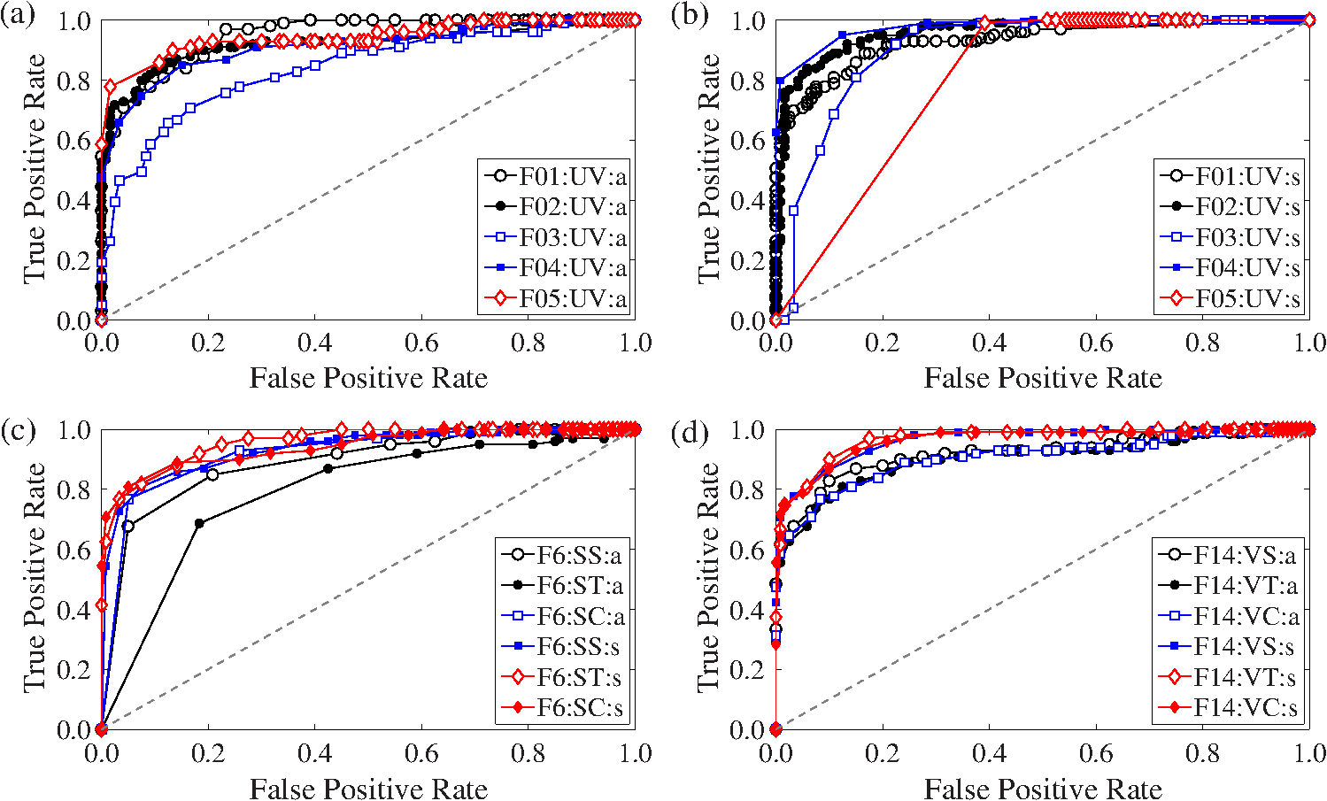

Fig. 11

Single feature classification results reported as the Youden index ( $Se + Sp - 1$ ) from ROC analysis for $μ_{a}$ (top two rows) and $μ_{s}^{'}$ (bottom two rows) features.

Of the 107 features that achieve $Y \geq 0.70$ , approximately 50% are from basic statistical features, 45% are from spatial Fourier analysis, and 5% are from GMM parameters. Over 47% of the features resulting in $Y \geq 0.70$ are derived from the variance across 2-D sagittal, transverse, and coronal planes (51 of the 107 features).

Basic features from $μ_{s}^{'}$ images are better classifiers than features from $μ_{a}$ images [Fig. 10(a) and 10(b)]. The variance of the unstructured data (F4:UV:s) is the best single feature classifier ( $Y = 0.82$ ) [Fig. 10(b)]. The absolute error between original images and GMM approximation performed strongly as one-dimensional (1-D) classifiers with up to $Y = 0.75$ [Fig. 10(c)]. The coefficients of the lowest order term of the 2-D-FFT of variance images (VS, VT, and VC) are very strong 1-D classifiers with up to $Y = 0.80$ [Fig. 10(d)].

4. Discussion and Conclusion

The goal of this 2-part paper is to establish a framework for diagnosing RA from DOT images. In this part (Part 1), we present a method for extracting features from DOT images that differentiate between subjects with and without RA. The process consists of three steps: (1) data pre-processing, (2) feature extraction, and (3) statistical and ROC curve analysis of individual features.

The framework is tested on 219 DOT images of PIP joints II to IV gathered through a clinical trial (33 subjects with RA and 20 healthy control subjects). Clinical diagnosis of RA according to the ACR criteria is the gold standard. Ultrasound and MRI scans of the clinically dominant hand were performed. A rheumatologist and a radiologist, in a blinded review, analyzed the images and classified each subject based on detectable symptoms of RA (groups B to E). Subjects without signs of RA-induced joint deformities were classified as healthy (group H) or as affected with RA (group $A$ ) based on nonimaging based evidence. A total of 596 features are extracted from the $μ_{a}$ and $μ_{s}^{'}$ reconstructions of all imaged joints. Statistical analysis of the extracted features is used to find features that reveal statistically significant differences between diagnosis groups.

Three important findings are discovered. First, through application of the nonparametric Kruskal–Wallis ANOVA test, we establish the existence of image features that show statistically significant differences between subjects with RA and without RA.

Second, we use Dunn’s test ( $p < 0.05$ ) to discover that features derived from group A (subjects with RA but without abnormal findings in MRI and ultrasound scans) are statistically different from features derived from healthy subjects (group H). At the same time, the differences in optical properties between group $A$ and groups $B$ to $E$ were generally not significant. This is an important finding because it shows that DOT imaging of PIP joints has the potential to detect the presence of RA even when ultrasound and MRI scans cannot detect effusion, synovitis, or erosion in the joint cavity.

Third, we discover that the $μ_{s}^{'}$ distribution yields stronger 1-D classifiers. ROC analysis shows three $μ_{s}^{'}$ features for which $Y \geq 0.8$ . This is a significant improvement over the previous work, where $Y \leq 0.59$ was obtained with ROC analysis.³ This represents the first time that $μ_{s}^{'}$ images are exploited to yield strong differences between PIP joints of subjects with and without RA. Additionally, we establish that the variance between sagittal, transverse, and coronal slices yields a large number of strong single feature classifiers ( $Y \geq 0.70$ ).

These three findings demonstrate that changes in optical properties induced by RA are detectable using DOT. The statistically significant differences between image features from affected and healthy subjects show that it might be possible to accurately diagnose RA using FD-DOT. Furthermore, the general lack of statistically significant differences between features from group $A$ and groups $B$ to $E$ is evidence that DOT is sensitive to changes in optical properties of the synovium that MRI and ultrasound cannot resolve.

The second part of this paper focuses on multidimensional classification using the features that result in the largest Youden indices from ROC analysis as presented in this study. Employing five different classification algorithms, we show that using multiple rather than single image features leads to higher sensitivities and specificities.

Acknowledgments

The authors would like to thank Julio D. Montejo for his contribution during the early stage of this project and Yrjö Häme for his assistance in implementing the feature extraction routines. This work was supported in part by a grant from the National Institute of Arthritis and Musculoskeletal and Skin Diseases (NIAMS-5R01AR046255), which is a part of the National Institutes of Health (NIH). Furthermore, L.D. Montejo was partially supported by a NIAMS training grant on “Multidisciplinary Engineering Training in Musculoskeletal Research ” (5 T32 AR059038 02).

References

1.

B. J. Tromberget al., “Assessing the future of diffuse optical imaging technologies for breast cancer management,” Med. Phys., 35 (6), 2443 –2451 (2008). http://dx.doi.org/10.1118/1.2919078 MPHYA6 0094-2405 Google Scholar

2.

A. V. Medvedevet al., “Diffuse optical tomography for brain imaging: continuous wave instrumentation and linear analysis methods,” Optical Methods and Instrumentation in Brain Imaging and Therapy, Springer, New York (2013). http://dx.doi.org/10.1016/j.brainres.2008.07.122 Google Scholar

3.

A. Hielscheret al., “Frequency-domain optical tomographic imaging of arthritic finger joints,” IEEE Trans. Med. Imag., 30 (10), 1725 –1736 (2011). http://dx.doi.org/10.1109/TMI.2011.2135374 ITMID4 0278-0062 Google Scholar

4.

L. D. Montejoet al., “Computer-aided diagnosis of rheumatoid arthritis with optical tomography, Part 2: image classification,” J. Biomed. Opt., 52 (6), 066012 (2013). CLCHAU 0009-9147 Google Scholar

5.

K. Doi, “Computer-aided diagnosis in medical imaging: historical review, current status and future potential,” Comput. Med. Imag. Graph., 31 (4–5), 198 –211 (2007). http://dx.doi.org/10.1016/j.compmedimag.2007.02.002 CMIGEY 0895-6111 Google Scholar

6.

A. P. G. LeilaH. EadieP. Taylor, “A systematic review of computer-assisted diagnosis in diagnostic cancer imaging,” Eur. J. Radiol., 81 (1), e70 –e76 (2012). http://dx.doi.org/10.1016/j.ejrad.2011.01.098 EJRADR 0720-048X Google Scholar

7.

K. Doi, “Current status and future potential of computer-aided diagnosis in medical imaging,” Br. J. Radiol., 78 3 –19 (2005). http://dx.doi.org/10.1259/bjr/82933343 BJRAAP 0007-1285 Google Scholar

8.

J. Shiraishiet al., “Computer-aided diagnosis for the classification of focal liver lesions by use of contrast-enhanced ultrasonography,” Med. Phys., 35 (5), 1734 –1746 (2008). http://dx.doi.org/10.1118/1.2900109 MPHYA6 0094-2405 Google Scholar

9.

L. A. Meinelet al., “Breast mri lesion classification: improved performance of human readers with a backpropagation neural network computer-aided diagnosis (cad) system,” J. Magn. Reson. Imag., 25 (1), 89 –95 (2007). http://dx.doi.org/10.1002/(ISSN)1522-2586 1053-1807 Google Scholar

10.

T. Arazi-Kleinmanet al., “Can breast mri computer-aided detection (cad) improve radiologist accuracy for lesions detected at mri screening and recommended for biopsy in a high-risk population?,” Clin. Radiol., 64 (12), 1166 –1174 (2009). http://dx.doi.org/10.1016/j.crad.2009.08.003 CLRAAG 0009-9260 Google Scholar

11.

K. DrukkerL. PesceM. Giger, “Repeatability in computer-aided diagnosis: application to breast cancer diagnosis on sonography,” Med. Phys., 37 (6), 2659 –2669 (2010). http://dx.doi.org/10.1118/1.3427409 MPHYA6 0094-2405 Google Scholar

12.

D. Newellet al., “Selection of diagnostic features on breast mri to differentiate between malignant and benign lesions using computer-aided diagnosis: differences in lesions presenting as mass and non-mass-like enhancement,” Eur. Radiol., 20, (4), 771 –781 (2010). http://dx.doi.org/10.1007/s00330-009-1616-y EURAE3 1432-1084 Google Scholar

13.

J. E. Levmanet al., “Effect of the enhancement threshold on the computer-aided detection of breast cancer using mri,” Acad. Radiol., 16 (9), 1064 –1069 (2009). http://dx.doi.org/10.1016/j.acra.2009.03.018 1076-6332 Google Scholar

14.

X. Qiet al., “Computer-aided diagnosis of dysplasia in barrett’s esophagus using endoscopic optical coherence tomography,” J. Biomed. Opt., 11 (4), 044010 (2006). http://dx.doi.org/10.1117/1.2337314 JBOPFO 1083-3668 Google Scholar

15.

F. Bazant-HegemarkN. Stone, “Towards automated classification of clinical optical coherence tomography data of dense tissues,” Lasers Med. Sci., 24 (4), 627 –638 (2009). http://dx.doi.org/10.1007/s10103-008-0615-6 LMSCEZ 1435-604X Google Scholar

16.

D. R. Buschet al., “Computer aided automatic detection of malignant lesions in diffuse optical mammography,” Med. Phys., 37 (4), 1840 –1849 (2010). http://dx.doi.org/10.1118/1.3314075 MPHYA6 0094-2405 Google Scholar

17.

J. Z. Wanget al., “Automated breast cancer classification using near-infrared optical tomographic images,” J. Biomed. Opt., 13 (4), 044001 (2008). http://dx.doi.org/10.1117/1.2956662 JBOPFO 1083-3668 Google Scholar

18.

X. Songet al., “Automated region detection based on the contrast-to-noise ratio in near-infrared tomography,” Appl. Opt., 43 1053 –1062 (2004). http://dx.doi.org/10.1364/AO.43.001053 APOPAI 0003-6935 Google Scholar

19.

X. Songet al., “Receiver operating characteristic and location analysis of simulated near-infrared tomography images,” J. Biomed. Opt., 12 (5), 054013 (2007). http://dx.doi.org/10.1117/1.2799197 JBOPFO 1083-3668 Google Scholar

20.

C. Zhuet al., “Model based and empirical spectral analysis for the diagnosis of breast cancer,” Opt. Express, 16 14961 –14978 (2008). http://dx.doi.org/10.1364/OE.16.014961 OPEXFF 1094-4087 Google Scholar

21.

T. M. Bydlonet al., “Performance metrics of an optical spectral imaging system for intra-operative assessment of breast tumor margins,” Opt. Express, 18 (8), 14961 –14978 (2010). http://dx.doi.org/10.1364/OE.18.008058 OPEXFF 1094-4087 Google Scholar

22.

C. D. Kloseet al., “Multiparameter classifications of optical tomographic images,” J. Biomed. Opt., 13 (5), 050503 (2008). http://dx.doi.org/10.1117/1.2981806 JBOPFO 1083-3668 Google Scholar

23.

C. D. Kloseet al., “Computer-aided interpretation approach for optical tomographic images,” J. Biomed. Opt., 15 (6), 066020 (2010). http://dx.doi.org/10.1117/1.3516705 JBOPFO 1083-3668 Google Scholar

24.

V. MajithiaS. A. Geraci, “Rheumatoid arthritis: diagnosis and management,” Am. J. Med., 120 (11), 936 –939 (2007). http://dx.doi.org/10.1016/j.amjmed.2007.04.005 AJMEAZ 0002-9343 Google Scholar

25.

C. G. Helmicket al., “Estimates of the prevalence of arthritis and other rheumatic conditions in the united states: part i,” Arthritis Rheum., 58 (1), 15 –25 (2008). http://dx.doi.org/10.1002/(ISSN)1529-0131 ARHEAW 0004-3591 Google Scholar

26.

A. Danielet al., “2010 Rheumatoid arthritis classification criteria: an american college of rheumatology/european league against rheumatism collaborative initiative,” Arthritis Rheum., 62 (9), 2569 –2581 (2010). http://dx.doi.org/10.1002/art.27584 ARHEAW 0004-3591 Google Scholar

27.

E. Solau-Gervaiset al., “Magnetic resonance imaging of the hand for the diagnosis of rheumatoid arthritis in the absence of anti-cyclic citrullinated peptide antibodies: a prospective study,” J. Rheumatol., 33 (9), 1760 –1765 (2006). JRHUA9 0315-162X Google Scholar

28.

J. H. BrownS. A. Deluca, “The radiology of rheumatoid arthritis,” Am. Fam. Physician, 52 (5), 1372 –1380 (1995). AFPYAE 0002-838X Google Scholar

29.

M. OstergaardM. Szkudlarek, “Imaging in rheumatoid arthritis—why mri and ultrasonography can no longer be ignored,” Scand. J. Rheumatol., 32 (2), 63 –73 (2003). http://dx.doi.org/10.1080/03009740310000058 SJRHAT 0300-9742 Google Scholar

30.

R. J. Wakefieldet al., “The value of sonography in the detection of bone erosions in patients with rheumatoid arthritis: a comparison with conventional radiography,” Arthritis Rheum., 43 (12), 2762 –2770 (2000). http://dx.doi.org/10.1002/1529-0131(200012)43:12<>1.0.CO;2-5 ARHEAW 0004-3591 Google Scholar

31.

J. Narvaezet al., “Usefulness of magnetic resonance imaging of the hand versus anticyclic citrullinated peptide antibody testing to confirm the diagnosis of clinically suspected early rheumatoid arthritis in the absence of rheumatoid factor and radiographic erosions,” Semin. Arthritis Rheum., 38 101 –109 (2008). http://dx.doi.org/10.1016/j.semarthrit.2007.10.012 SAHRBF 0049-0172 Google Scholar

32.

K. RenG. BalA. H. Hielscher, “Transport- and diffusion-based optical tomography in small domains: a comparative study,” Appl. Opt., 46 6669 –6679 (2007). http://dx.doi.org/10.1364/AO.46.006669 APOPAI 0003-6935 Google Scholar

33.

A. D. Klose, “Radiative transfer of luminescence light in biological tissue,” Light Scattering Reviews 4, 293 –345 Springer Berlin Heidelberg, Germany (2009). Google Scholar

34.

S. TheodoridisK. Koutroumbas, Pattern Recognition, Elsevier/Academic Press, Massachusetts, USA (2006). Google Scholar

35.

S. Glantz, Primer of Biostatistics, 6th ed.McGraw-Hill Medical Pub. Division(2005). Google Scholar

36.

S. KillipZ. MahfoudK. Pearce, “What is an intracluster correlation coefficient? Crucial concepts for primary care researchers,” Ann. Fam. Med., 2 (3), 204 –208 (2004). http://dx.doi.org/10.1370/afm.141 1544-1709 Google Scholar

37.

A. DonnerJ. J. Koval, “The estimation of intraclass correlation in the analysis of family data,” Biometrics, 36 (1), 19 –25 http://dx.doi.org/10.2307/2530491 BIOMB6 0006-341X Google Scholar

38.

E. B. Wilson, “Probable inference, the law of succession, and statistical inference,” J. Am. Stat. Assoc., 22 (158), 209 –212 (1927). http://dx.doi.org/10.1080/01621459.1927.10502953 JSTNAL 0003-1291 Google Scholar

39.

H. Ahrens, “Multivariate variance–covariance components (mvcc) and generalized intraclass correlation coefficient (gicc),” Biom. Z., 18 (7), 527 –533 (1976). http://dx.doi.org/10.1002/(ISSN)1521-4037 BIZEB3 0006-3452 Google Scholar

40.

M. H. ZweigG. Campbell, “Receiver-operating characteristic (ROC) plots: a fundamental evaluation tool in clinical medicine,” Clin. Chem., 39 (4), 561 –577 (1993). CLCHAU 0009-9147 Google Scholar

Citation Download Citation

Ludguier D. Montejo, Jingfei Jia, Hyun K. Kim, Uwe J. Netz, Sabine Blaschke, Gerhard A. Mueller, and Andreas H. Hielscher "Computer-aided diagnosis of rheumatoid arthritis with optical tomography, Part 1: feature extraction," Journal of Biomedical Optics 18(7), 076001 (15 July 2013). https://doi.org/10.1117/1.JBO.18.7.076001

Published: 15 July 2013

Access the abstract

JOURNAL ARTICLE
14 PAGES

DOWNLOAD PAPER SAVE TO MY LIBRARY

GET CITATION

CITATIONS

Cited by 28 scholarly publications.

Explore citations on Lens.org

RIGHTS & PERMISSIONS

Get copyright permission Get copyright permission on Copyright Marketplace

KEYWORDS

Computer aided diagnosis and therapy

Feature extraction

Magnetic resonance imaging

Selenium

Data modeling

Optical tomography

Ultrasonography

1.

Introduction

1.1.

Overview

1.2.

Background

2.

Methods

2.1.

Clinical Study

2.1.1.

Rheumatoid arthritis

2.1.2.

Clinical data

Table 1

Fig. 1

Fig. 2

2.2.

Data Pre-processing

Fig. 3

Eq. (1)

Eq. (2)

Table 2

Fig. 4

2.3.

Feature Extraction

2.3.1.

Basic features

Table 3

2.3.2.

Gaussian mixture model parameterization of absorption and scattering maps

Eq. (3)

Fig. 5

Table 4

2.3.3.

Spatial frequency coefficients

Fig. 6

Table 5

2.3.4.

Short-hand notation

2.4.

Statistical Analysis

2.4.1.

Kruskal–Wallis ANOVA test and Dunn’s test

2.4.2.

Effective sample size

Eq. (4)

Eq. (5)

Eq. (6)

Eq. (7)

Eq. (8)

2.4.3.

ROC analysis

3.

Results

3.1.

Parameterization and Spatial-Frequency Analysis

Fig. 7

3.2.

Kruskal–Wallis ANOVA

Fig. 8

3.3.

Dunn’s Test

Table 6

Fig. 9

3.4.

ROC Analysis

Fig. 10

Fig. 11

4.

Discussion and Conclusion

Acknowledgments

References

Show All Keywords

Keywords/Phrases

Search In:

Publication Years