|
|
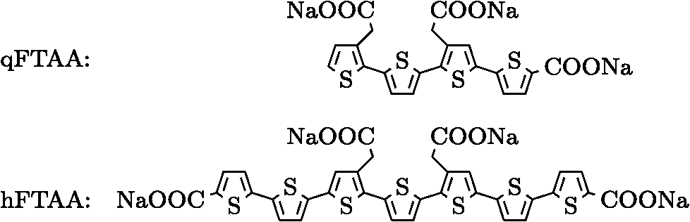
1.IntroductionModern fluorescence microscopes are capable of recording images with a reasonably resolved spectrum in each pixel, enabling advanced spectroscopic characterization of optically resolved structures. However, this requires access to adequate methods for resolving and discriminating spectral features or components of the generated hyperspectral images. There are several methods for accomplishing this, and they have become more and more sophisticated with the increase in computing power available in modern computers. One common way of doing spectral analysis is by linear spectral unmixing,1–3 which classifies the measured spectrum in every pixel in terms of a linear sum of input references. If the reference spectra are not known, a commonly used method is the principal component analysis,4 which separates the spectrum into its main (orthogonal) components, using statistics gathered from the image. Another approach that classifies the spectra is the spectral angle mapper algorithm.5–7 All of these methods have their drawbacks, e.g., they are difficult to use if the signals are weak with interfering background fluorescence or if there are large differences in relative quantum efficiency of different spectral components. The problems associated with the common signal processing tools prompted us to propose a spectral cross-correlation algorithm for hyperspectral images.8 The correlation coefficient8 is advantageous over, for instance, linear spectral unmixing,1–3 since it is statistically defined and scale invariant. It is limited to between and 1, with being , 0 and 1 . In spectral measurements, the measured intensities should never be negative, as intensity is dependent on the number of photons. As a result, the correlation coefficient should be larger than 0, assuming the background offset is reasonably small. Due to random noise in the measurement, the correlation coefficient will never be exactly 1. As will be shown, this method is well suited for the analysis of biological samples with a complex background as we can gain sensitivity by using all spectral ranges of the hyperspectral image, but we are at the same time able to discriminate the relative contribution from different spectral components as with the linear signal processing algorithms. As a demonstration of the correlation algorithm,8 we here present a detailed analysis of double-staining experiments of Alzheimer’s disease (AD) progression in mouse models. AD is known to be accompanied by the accumulation of peptide deposits in the brain, although the relation to the disease is still in many respects unknown. Luminescent-conjugated oligothiophenes (LCOs)9 and the related polymers10,11 are known to bind to amyloid deposits and change its fluorescence emission, enabling spectral diagnostics of plaque formation.12 Smaller variants of LCOs can be used in vivo as they pass the blood–brain barrier.13 It was recently shown by Nyström et al.,14 that simultaneous staining with two different LCOs reveals varying spectral characteristics based on structural differences of the formed protein aggregates. Central plaque regions appear to have larger spectral contribution from the shorter of the two LCOs, quadro-formylthiophene acetic acid (qFTAA), whereas the longer hepta-formylthiophene acetic acid (hFTAA), known to be more promiscuous and stain both prefibrilar aggregates and mature amyloid deposits, was shown to stain plaques from the different ages more uniformly. The results were compared with in vitro fibrillation experiments and it was shown that the spectral characteristics of the two LCOs were related to the time point of the fibrillation process. Another study based on classification using spectral angle mapping by Wegenast-Braun et al.15 confirmed the location of the LCO (hFTAA) to the plaques, and compared it to other conventional staining methods based on antibodies, Congo red, methoxy-X04, and thioflavin S. The previous study by Nyström et al.14 for characterization of age-dependent conformational rearrangements of the deposits in AD relied on a rather simple comparison of two spectral components in the center of the doubly stained AD plaques. By using the correlation algorithm and developing auxiliary routines for plaque analysis, such as radial distribution analysis, we can obtain a wealth of detailed structural data. Here, we apply the cross-correlation algorithm and make a statistical analysis of relative fluorescence stain distribution of the same set of raw data as used in the study of Nyström et al.14 Based on the correlation analysis, we make a detailed comparison between AD mice of different ages in a systematic manner to reveal further details of the progression of AD amyloid plaque formation in such mouse models. 2.Materials and Methods2.1.SamplesThe LCO staining solution, containing a mix of qFTAA and hFTAA, was prepared by using stock solutions prepared in 2 mM NaOH and stored at 4°C while awaiting use. Synthesizing of qFTAA and hFTAA was done as described by Klingstedt et al.9 Before staining, fresh solutions were prepared by diluting the stock to in phosphate buffered saline (PBS). Then qFTAA and hFTAA were mixed in a ratio of , resulting in a final concentration of 2.4 μM qFTAA and 0.7 μM hFTAA, in assay solutions. Brain tissues from 19 mice aged 6 to 23 months were employed in the study to facilitate the investigation of the age dependence of spectral variations in the plaques. About 10 μm cryo sections were prepared and kept at −20°C until needed. The LCO staining solution containing a mix of qFTAA and hFTAA was applied to the cryosections. The sections were washed with PBS and mounted with Dako fluorescence mounting medium. The slides were left in room temperature in the dark overnight and sealed with nail polish. Structures for qFTAA and hFTAA can be seen in Fig. 1. See Nyström et al. for further details.14 2.2.Hyperspectral ImagingAfter preparation, the samples were imaged using a Leica DM6000 B fluorescence microscope mounted with a SpectraCube module from applied spectral imaging (ASI). An excitation wavelength filter with peak transmission at 405 nm and a full width at half maximum of and a long-pass filter allowing emission above 450 nm were used to block back-propagating light from the excitation. 2.3.Correlation AnalysisThe correlation analysis, see Ellingsen et al. for the details,8 is based on calculating the cross-correlation coefficient between the measured spectrum in a pixel () and a reference spectra (). This is repeated for every pixel in the hyperspectral image above a certain background threshold, yielding a new image with the correlation coefficient. If there are additional reference spectra, the process is repeated, yielding one correlation image for each reference spectrum. For the remainder of this work, the correlation coefficient will be referred to as the correlation. 3.Results and Discussion3.1.General Approach for Collecting DataHyperspectral images were recorded using the fluorescent microscope (Leica) equipped with an ASI Sagnac interferometric hyperspectral imager, see Sec. 2.2 for details. The initial hyperspectral images, each containing several plaques, were thresholded to remove background (signal to noise of more than 10 for the intensity image, with the same level for individual spectral channels) and then the data of individual plaques were extracted using operator selected region of interest (ROI). Figure 2 shows an example of the thresholded image and Fig. 3 shows a resulting cropped image. Fig. 2Intensity image (sum over spectrum) with regions of interest showing the seven cropped areas used in the rest of the analysis. Color scale is in counts. The threshold of 3500 counts is shown as dark blue. The mouse age was 686 days.  Fig. 3Intensity image of crop number 7 in Fig. 2 colored in the natural colors of the eye using the algorithm described in Ref. 16. (See Video 1 MPEG, 0.8 MB) [URL: http://dx.doi.org/10.1117/1.JBO.18.10.101313.1] for a wavelength scan over the image.  Totally, 19 different AD mice were examined and data were collected from between 5 and 34 plaques (with majority of them above 20) for each age (some mice showed more plaques than others). Correlation images were then generated from this set of raw data using reference spectra from plaques stained with pure qFTAA and hFTAA, respectively. The two reference spectra are shown in Fig. 4. For more details on the acquisition of these spectra, see Nyström et al.14 As can be seen in Fig. 4, the references are well defined, with distinct spectral differences. When mixed and used in double staining the resulting spectra will be harder to separate due to the occurrence of both stains and a background that can vary depending on the location within the sample and the sample itself. Qualitative observation of plaques generally showed a diffuse structure surrounding a region of high fluorescence, defining a center of high fluorescence intensity. The plaque shapes were not distinct but essentially circular with small elliptical distortions, or with patches of smaller regions with high intensities arranged around an essentially circular main plaque. Two ways of identifying the plaque center was tested: (1) from the average of some pixels of highest intensity, or (2) by calculating the center of mass for the whole intensity distribution, see e.g., Adams.17 The latter approach was abandoned as it generated a much larger spread of data when calculating radial distributions, especially with plaques that were far from spherical. Therefore, approach (1) was adopted by defining a threshold for the background intensity (sum over the spectrum) image, and then finding the maximum after passing it through a median filter. The motivation for adopting this approach was that the plaques are actually sections of three-dimensional structures. A consequence would then be that the center would be the area where the plaque is “thickest” and therefore the fluorescence intensity should be the highest. Using a median filter ensures that a singular pixel with a high intensity, e.g., from noise or a measurement error, was not chosen as the center. An example of such a defined center is shown in Fig. 5 for a plaque that is very irregular in shape. The choice of method for finding the center for any of the methods will give some results where the center is ill-defined; however, owing to the nature of the statistical analysis, as long as the majority of the centers are found well enough, the overall results from the statistics should make the most probable distribution most significant. Fig. 5Image showing the sum over the spectrum for crop number 7 in in Fig. 2. The white plus in the figure marks the center used in the radial analysis. Color scale is in counts. The threshold of 3500 counts is shown as dark blue. 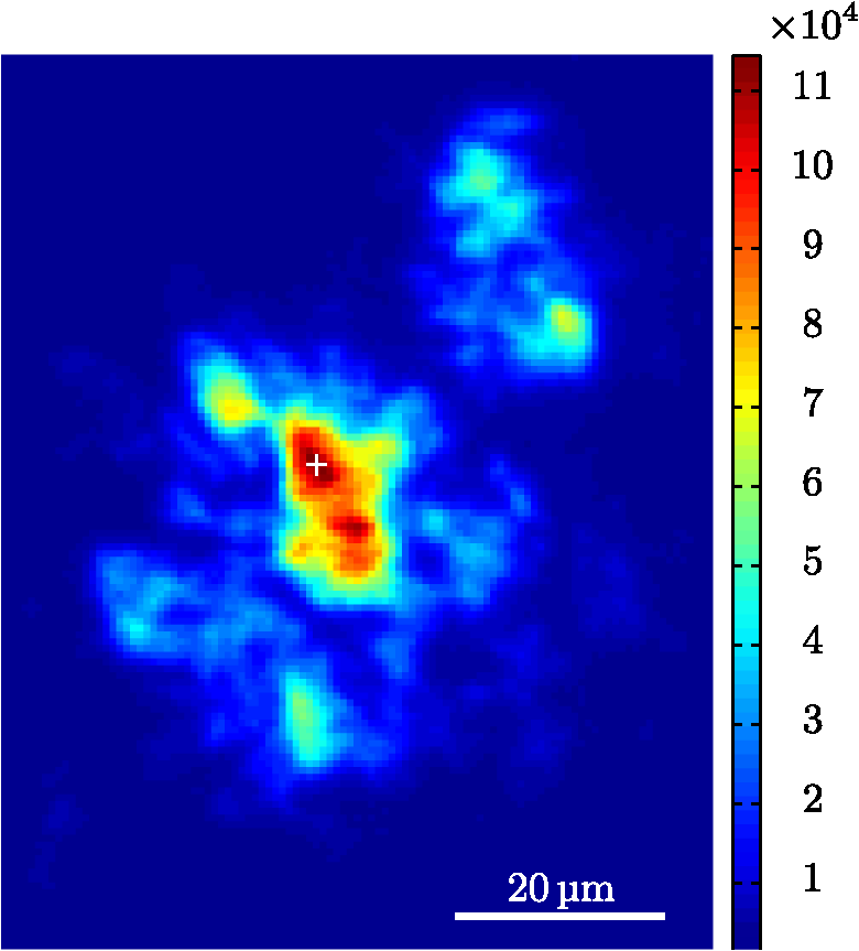 After the correlation images for all the plaques were generated, (see representative correlation images for the two stains in Fig. 6), the data set was further analyzed in terms of radial distribution and mouse age. Fig. 6Image showing the correlation between the qFTAA (left) or hFTAA (right) reference and the measured spectrum. The crop is the same as Fig. 5. Notice the big difference in the center of the plaque between the correlation value. The threshold of 3500 counts is shown as dark blue. 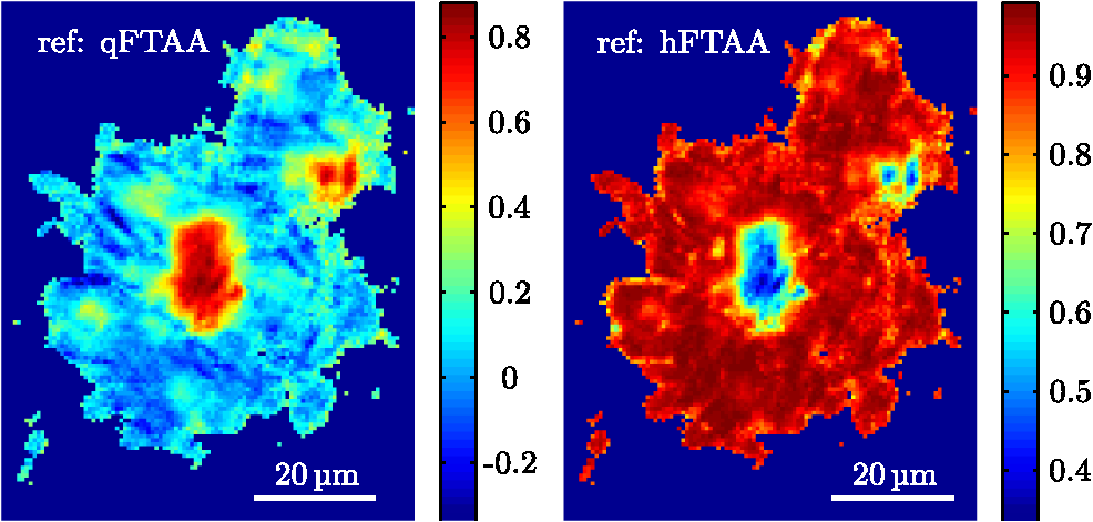 3.2.Spectral Correlations Versus Radial DistributionHaving calculated the correlation for every pixel in an image, we now want to map its distribution, e.g., the radial distribution within a plaque. The distance or radius from the plaque center is given by where is the center as discussed in Sec. 3.1 and represents the coordinate of a given pixel in the image. The value of the radius is rounded to an integer, and all of the valid pixels (those above the background threshold) are sorted into bins according to their integer value, enabling the plotting of correlation as a function of radius for each correlation distribution. As the goal was to compare different plaques with different sizes (due to, for instance, age, sample preparation, and imaging), the radius needed to be normalized. This was done by distributing the radii onto 21 uniformly spaced radii between 0 and 1. This is equivalent to dividing the radius by the maximum and then re-sampling the data to 21 points from a much higher number of points. With a normalized radius, it was possible to do statistics for the correlation of each mouse as a function of plaques radius. Four of these statistical plots, showing the mean and standard deviation as a function of radius, are shown in Fig. 7. These plots are not randomly selected, rather they are the most clear examples of the progression of the radial distribution as a function of mouse age: Figs. 6 and 7 clearly show that qFTAA stains the center of a plaque much better than the periphery. For hFTAA the situation is opposite, with the highest values in the periphery and the smallest in the center.Fig. 7The mean correlation and its standard deviation as a function of normalized distance from center (radius) for four mice of different ages. The mean and standard deviation are calculated over all analyzed plaques of each mouse. The age is indicated in each plot.  The findings so far are in agreement with the simple analysis in Nyström et al.14 based on a simple comparison of intensities of two spectral emission peaks in the center of a plaque, where the peak at 500 nm corresponds to the binding of qFTAA and the peak at 540 nm reflects the binding of hFTAA. The difference between the two references becomes even more pronounced the older the mice are, with the correlation eventually crossing each other somewhere around 400 days (see Fig. 7). From this, it can be deducted that there is a clear change over time with respect to the structure of the plaque, clearly inhibiting the binding of hFTAA in the center. Since the LCOs are sensitive to the conformation of the proteins within the plaque, this yields a very promising result for the study of structural changes within the plaque for different ages. Further details of the spectral correlation was obtained from a statistical analysis of all plaques, to be discussed below (Sec. 3.3). 3.3.Statistical Analysis of Spectral DistributionIn addition to the four mouse ages shown in Fig. 7, data of 15 more AD mice were recorded, correlated with the references and the corresponding radial characteristics was calculated for each age. In order to plot the wealth of analyzed data, the relative abundance of the hFTAA and qFTAA spectral components are plotted as a function of mouse age at different relative radii as in Fig. 8. Hereby, we obtain an overview of the spectral characteristics for the essential regions of the plaques. This shows that the correlation for qFTAA and hFTAA in the plaque center varies significantly as a function of age, apparently crossing each other for mice at approximately 340–490 days of age. In the outer regions of the plaques (Fig. 8: lower panels), the relative abundance is relatively constant up to approximately 500 days of age. Here, hFTAA has a much larger propensity to bind with a correlation value close to 1. These results and conclusions are in agreement with the simpler analysis in Nyström et al.14 Interestingly, the correlation analysis shows a pronounced “second wave” as qFTAA increases its correlation value in the outer regions above 500 days. Also, a second crossing of the correlation values is prominent at plaque center (Fig. 8: upper left panel), indicating that there are different structural properties of plaques in the younger mice ( days) compared with the older ones, and that hFTAA staining starts to dominate the plaque centers again at days. These results and conclusions are in agreement with the simpler analysis in Nyström et al.14 Variation in plaque morphologies in both man18 and mouse12 has been documented earlier. However, our described method allows for both qualitative and quantitative analysis of images from biological specimens due to the ability to analyze the entire image for a series of images in a data set. Together with the ability to analyze radial distributions and smaller spectral differences, it provides a more detailed and accurate approach, with statistically verified results. Fig. 8Mean correlation as a function of age in days and normalized distance from the center. Notice that the -axis (age) is uniformly spaced with respect to each case, and that there are three identical ages (245, 392, 531 days) which are from different mice and therefore are shown as different points. The outer red/blue borders denote the standard deviation.  4.ConclusionThis paper shows the application of spectral correlation on hyperspectral images obtained from samples of double-stained amyloid plaques of AD mice brain sections. Using the spectral correlation approach, we obtain a wealth of signal processing results that can be used to assess the structural composition leading to spectral changes in detail. In agreement with a previous study based on a simple two spectral point comparison,14 it is found that there are structural changes within the plaques for AD mice of different ages. Using our analysis strategy, these spectral changes could be quantified in detail and it was found that the radical distribution of relative abundance showed a clear monotonous change in AD mice up to about 500 days of age. Moreover, a second transition in terms of plaque inhomogeneity was observed for mice of very old age ( days) and this may suggest further detailed studies of AD mouse models at high ages. Conclusively, the spectral correlation algorithm was demonstrated as useful in the assessment of fluorescence hyper spectral images in multiple staining experiments. AcknowledgmentsThis work was supported by the EU-FP7 Health Programme Project LUPAS ( www.lupas-amyloid.eu). In addition, Sofie Nyström was supported by the Swedish Alzheimer Foundation. We acknowledge the members of the LUPAS consortium for discussions and samples used for testing the cross-correlation method. In particular, we acknowledge Susann Handrick and Bettina Wegenast-Braun for assisting in sample preparations and Profs, Per Hammarström, Peter Nilsson, Christian Liebig, Frank Heppner, and Mathias Jucker for valuable discussions. ReferencesM. E. Dickinson,
“Multi-spectral imaging and linear unmixing add a whole new dimension to laser scanning fluorescence microscopy,”
Biotechniques, 31
(6), 1272
–1278
(2001). BTNQDO 0736-6205 Google Scholar
T. Zimmermann,
“Spectral imaging and its applications in live cell microscopy,”
FEBS Lett., 546
(1), 87
–92
(2003). http://dx.doi.org/10.1016/S0014-5793(03)00521-0 FEBLAL 0014-5793 Google Scholar
T. Zimmermann,
“Spectral imaging and linear unmixing in light microscopy,”
Microsc. Tech., 95 245
–265
(2005). http://dx.doi.org/10.1007/b102216 MRTEEO 1059-910X Google Scholar
I. T. Jolliffe, Principal Component Analysis, 2nd ed.Springer-Verlag, New York
(2002). Google Scholar
O. A. De CarvalhoP. R. Meneses,
“Spectral correlation mapper (SCM): an improvement on the spectral angle mapper (SAM),”
in Airborne Visible/Infrared Imaging Spectrometer (AVIRIS) 2000 Workshop Proceedings,
(2000). Google Scholar
P. E. DennisonK. Q. HalliganD. A. Roberts,
“A comparison of error metrics and constraints for multiple end member spectral mixture analysis and spectral angle mapper,”
Rem. Sens. Environ., 93
(3), 359
–367
(2004). http://dx.doi.org/10.1016/j.rse.2004.07.013 RSEEA7 0034-4257 Google Scholar
H. Z. M. ShafriA. SuhailiS. Mansor,
“The performance of maximum likelihood, spectral angle mapper, neural network and decision tree classifiers in hyperspectral image analysis,”
J. Comput. Sci., 3
(6), 419
–423
(2007). http://dx.doi.org/10.3844/jcssp.2007.419.423 1549-3636 Google Scholar
P. G. Ellingsenet al.,
“Hyperspectral analysis using the correlation between image and reference,”
J. Biomed. Opt., 18
(2), 20501
(2013). http://dx.doi.org/10.1117/1.JBO.18.2.020501 JBOPFO 1083-3668 Google Scholar
T. Klingstedtet al.,
“Synthesis of a library of oligothiophenes and their utilization as fluorescent ligands for spectral assignment of protein aggregates,”
Org. Biomol. Chem., 9
(24), 8356
–70
(2011). http://dx.doi.org/10.1039/c1ob05637a OBCRAK 1477-0520 Google Scholar
K. P. R. Nilssonet al.,
“Conjugated polyelectrolytes–conformation-sensitive optical probes for staining and characterization of amyloid deposits,”
Chembiochem: Eur. J. Chem. Biol., 7
(7), 1096
–104
(2006). http://dx.doi.org/10.1002/cbic.v7:7 CBCHFX 1439-4227 Google Scholar
F. Stabo-Eeget al.,
“Quantum efficiency and two-photon absorption cross-section of conjugated polyelectrolytes used for protein conformation measurements with applications on amyloid structures,”
Chem. Phys., 336
(2–3), 121
–126
(2007). http://dx.doi.org/10.1016/j.chemphys.2007.06.020 CMPHC2 0301-0104 Google Scholar
K. P. R. Nilssonet al.,
“Imaging distinct conformational states of amyloid-beta fibrils in Alzheimer’s disease using novel luminescent probes,”
ACS Chem. Biol., 2
(8), 553
–560
(2007). http://dx.doi.org/10.1021/cb700116u ACBCCT 1554-8929 Google Scholar
A. Aslundet al.,
“Novel pentameric thiophene derivatives for in vitro and in vivo optical imaging of a plethora of protein aggregates in cerebral amyloidoses,”
ACS Chem. Biol., 4
(8), 673
–684
(2009). http://dx.doi.org/10.1021/cb900112v ACBCCT 1554-8929 Google Scholar
S. Nyströmet al.,
“Evidence for age dependent in vivo conformational rearrangement within amyloid deposits,”
ACS Chem. Biol., 8
(6), 1128
–1133
(2013). https://doi.org/10.1021/cb4000376 ACBCCT 1554-8929 Google Scholar
B. M. Wegenast-Braunet al.,
“Spectral discrimination of cerebral amyloid lesions after peripheral application of luminescent conjugated oligothiophenes,”
Am. J. Pathol., 181
(6), 1953
–1960
(2012). http://dx.doi.org/10.1016/j.ajpath.2012.08.031 AJPAA4 0002-9440 Google Scholar
R. L., ,
“Conversion of wavelength in nanometers to RGB in Python,”
Coding Mess,
(2009) http://codingmess.blogspot.no/2009/05/conversion-of-wavelength-in-nanometers.html , May 2013). Google Scholar
R. A. Adams, Calculus: A Complete Course, 432
–437 5th ed.Addison-Wesley, Toronto
(2003). Google Scholar
L.-W. Jinet al.,
“Imaging linear birefringence and dichroism in cerebral amyloid pathologies,”
Proc. Natl. Acad. Sci. U. S. A., 100
(26), 15294
–15298
(2003). http://dx.doi.org/10.1073/pnas.2534647100 1091-6490 Google Scholar
|