1.

Introduction

Diffuse optical tomography (DOT) is a volumetric optical imaging technique that relies on modeling light transport in tissue using the diffusion approximation, which is generally applicable in scatter dominated systems. The spectral measure of the diffuse transport of near-infrared light through soft tissue can provide the ability to image functional tissue information such as hemoglobin oxygenation and water fraction, which can be useful as a noninvasive means of identifying cancer.^1–3 This method has also been proven successful by the use of luminescence probes using, for example, fluorescence markers to allow quantitative molecular imaging of functional exogenous reporters.^4,5 Light modeling can be done analytically,⁶ providing high accuracy and computational speed, but only on simple and dominantly homogeneous geometries. Numerical approaches allow solutions to be computed for more complex geometries, but require more computational time as well as a discrete representation (volume mesh) of the domain.^7,8 Due to the generally poor spatial resolution of DOT, the prevailing trend in the field is toward combining it with other imaging modalities and incorporating high-resolution tissue structural information in the image recovery algorithm. Notable examples of this include computed tomography (CT) or magnetic resonance imaging (MRI)-guided DOT, and these techniques provide the potential for increased accuracy.^9–12 Although the details of finite-element-based methods for modeling light transport in tissue are well covered in literature,^13–21 the computational packages available for such modeling have until now included quite limited mesh creation tools or no mesh creation tools at all. In this work, an integrated and freely available software package is outlined and tested, which allows users to go all the way from import of standard digital imaging and communications in medicine (DICOM) images (and other related formats) to segmentation and meshing, and through to light simulation and property recovery. Image-guided DOT is very dependent on the ability to easily produce high-quality three-dimensional (3-D) volume meshes from medical images, and the process of mesh creation is a significantly underappreciated but complex issue, which is directly solved in many cases by software such as this.

The software tool developed at Dartmouth College and University of Birmingham, United Kingdom, called Nirfast, is a finite-element-based package for modeling near-infrared light transport in tissue for medical applications.^22,23 It is open source, free, and cross platform as developed under MATLAB (Mathworks Inc.), which also allows user-friendly understanding and modifications. Applications of Nirfast are diverse, including optical modeling for small animal imaging,^24–27 breast imaging,³ brain imaging,^28,29 and light dose verification in photodynamic therapy of the pancreas.

Accurate diffusion modeling in optical tomography requires a 3-D geometry since the photon scattering is in all directions.²⁰ Since the core finite element method (FEM) code of Nirfast is based on MATLAB,²² this has in the past hindered its ability to allow for easy coupling to highly complex 3-D meshing tools. One issue stems from the inability of MATLAB to efficiently visualize large 3-D meshes, while another issue is the necessity for custom image processing tools when dealing with an assortment of different medical image types and formats. Using a visualization toolkit/insight segmentation and registration toolkit-based platform, which itself is an open-source application, for segmentation and meshing has helped to address these issues by providing a seamless coupling within Nirfast. Providing the tools and workflow needed to create an FEM mesh from a variety of different types of medical images and seamlessly using this mesh for light transport modeling are essential to making DOT accessible and useful.

The current version of Nirfast includes full-featured segmentation and mesh creation tools for quickly and easily creating high-quality 3-D finite-element meshes from medical images.²³ The segmentation tools have been developed in collaboration with Kitware Inc. (Clifton Park, NY). Creating suitable volumetric meshes of complex tissue geometries is a particular challenge for multimodal DOT, due to the variety of contrast characteristics present in different imaging modalities and tissue types/models. Manual manipulation of the segmentation and mesh creation process often requires an overwhelming time investment, and high mesh element quality is notoriously difficult to ensure. It is also very important to retain both the outer and inner region surfaces (internal boundaries) in a mesh to allow the application of prior knowledge for both the forward and inverse models. Segmentation is rarely fully automated because some manual manipulation or input is standard for many complex problems, but by providing a customized collection of semiautomated routines, it is possible to substantially reduce the amount of manual touch-up required. There are various mesh creation tools available either commercially or freely, but each has its own limitations in application to optical tomography. For example, MeshLab is an open-source tool for creating unstructured 3-D triangular meshes, but has no semiautomated segmentation routines³⁰ and is also lacking some workflow features such as the ability to undo the last action. Mimics is a commonly used commercial package designed for medical image processing, but mesh creation requires a great deal of manual input, and it has difficulty with multiple-region problems.³¹ Netgen is a freely available 3-D tetrahedral mesh generator, but has limitations with multiple-region problems.³² Some other mesh creation tools include DistMesh,³³ iso2mesh,³⁴ and quality mesh generation,³⁵ but these are not linked to segmentation tools per se. There is no freely available tool that incorporates all of the workflow elements needed for segmentation and mesh creation in optical tomography in a seamless manner. The new tools in Nirfast help to address these issues, and in this study, their capabilities are tested and quantified in a series of cases which are representative of key application areas.

2.

Materials and Methods

The segmentation and mesh creation tools in Nirfast allow for a variety of different inputs, including standard DICOM formats for medical images, general image formats (stacks of bmp, jpg, png, etc.), and structured geometry formats (vtk, mha, etc.). It can be used for a variety of different medical imaging modalities, such as CT, MR, ultrasound, and microCT. Both automatic and manual means of segmenting these images have been provided, and mesh creation is fully automated with customizable parameters.

The capability of these tools is demonstrated on four different cases that are relevant to the modeling of light propagation in tissue and optical tomography: small animal imaging, breast imaging, brain imaging, and light dose modeling in photodynamic therapy of the pancreas. The small animal example used a stack of CT images of the front portion of a mouse, consisting of 30 axial slices of 256 by 256 pixels, with a slice thickness of 0.35 mm. The images were taken on a Phillips MR Achieva medical system, in the form of a DICOM stack. The breast example used a stack of T1-weighted MR images, consisting of 149 coronal slices of 360 by 360 pixels, with a slice thickness of 0.64 mm. The images were taken on a Phillips MR Achieva medical system, in the form of a DICOM stack. The brain example used a stack of T1-weighted MR images, consisting of 256 axial slices of 256 by 256 pixels, with a slice thickness of 1 mm. The images were taken on a Siemens Trio 3T scanner and are stored in .hdr and .img files. The pancreas example used a stack of arterial phase CT images, consisting of 90 axial slices of 512 by 512 pixels, with a slice thickness of 1 mm. The images were taken on a Seimens Sensation 64 CT system, in the form of a DICOM stack. In each case, the appropriate modules were used to maximize the quality of the resulting mesh and increase the speed of the entire process.

The general procedure for processing the images follows: First, the medical images are imported into the segmentation interface, shown in Fig. 1. Next, automatic segmentation modules are used to identify different tissue types and regions as accurately as possible. See Table 1 for the steps used in each case, as well as parameter values. The modules and their respective parameters are detailed in Table 2. Explanations of the major segmentation modules are described below.

Fig. 1

The interface for segmentation of tissue types in medical images is shown, with 3-D orthogonal views at right and histogram information at left.

Table 1

Time benchmarks for the segmentation and mesh creation of four different imaging cases: brain, pancreas, breast, and small animal, with the key steps in accurate segmentation identified and the time required for each step specified.

Table 2

List of automated segmentation modules available for identifying tissue types, including an explanation of the parameters in each case.

The iterative hole-filling algorithm classifies small volumes within a larger region as part of the outer region. In each iteration, a voting algorithm determines whether each pixel is filled based on the percentage of surrounding pixels that are filled, a ratio defined as the majority threshold.³⁶ The number of iterations controls the maximum size of holes and cavities filled. This is useful as a final step for any segmentation, to ensure that each tissue type region is homogeneous and lacking unintended holes. The K-means and Markov random field module performs a classification using a K-means algorithm to cluster grayscale values and then further refines the classification by taking spatial coherence into account.³⁷ The refinement is done with a Markov random field algorithm. The essential minimization function governing this module is given below, where $x$ is the set of grayscale values, $S$ is the $k$ sets of classification groups, and $u$ is the set of mean values in each $S$.

After automatic segmentation, the regions are manually touched up using a paintbrush in order to fix any remaining issues with the segmentation such as stray pixels or holes. Finally, the segmentation is provided as an input to the meshing routine, which creates a 3-D tetrahedral mesh from the stack of two-dimensional (2-D) masks in a single run. This eliminates intermediate steps such as creating 3-D surfaces and thus requires less mesh preprocessing. The resulting mesh is multiregional and can preserve the structural boundaries of segmented tissues. The user has control over element size, quality, and approximation error. For ease of use, these values are set automatically based on the segmentation and medical image information, and no prior knowledge of mesh generation is required to use the tool.

The volume meshing algorithm is unique and based on the computational geometry algorithms library (CGAL)⁴² and consists of several new features and implementations that are briefly outlined. The CGAL mesh generation libraries are based on a meshing engine utilizing the method of Delaunay refinement.⁴³ It uses the method of restricted Delaunay triangulation to approximate one-dimensional curved features and curved surface patches from a finite set of point samples on a surface^44,45 to achieve accurate representation of boundary and subdividing surfaces in the mesh. One very important feature that is of importance is that the domain to be meshed is a region of 3-D space that has to be bounded and the region may be connected or composed of multiple components and/or subdivided in several subdomains. The flexibility of this volume meshing algorithm allows the creation of 3-D volumes consisting of several nonoverlapping regions, allowing the utilization of structural prior information in diffuse optical imaging. The output mesh includes subcomplexes that approximate each input domain feature as defined in the segmented mask described above. During the meshing phase, several parameters can be defined to allow optimization of 3-D meshing, consisting of surface facet settings and tetrahedron size, which are detailed in Table 3.

Table 3

List of parameters controlling the 3-D tetrahedral mesh creation, including description of the function of each parameter.

Once the volumetric mesh has been created, a new feature has been added to allow the users to further optimize the 3-D mesh utilizing the Stellar mesh improvement algorithm.⁴⁶ This optimization routine improves tetrahedral meshes so that their worst tetrahedra have high quality, making them more suitable for finite element analysis. Stellar employs a broad selection of improvement operations, including vertex smoothing by nonsmooth optimization, stellar flips and other topological transformations, vertex insertion, and edge contraction. If the domain shape has no small angles, Stellar routinely improves meshes so that the smallest dihedral angle is $>30\mathrm{deg}$ and the largest dihedral angle is $<140\mathrm{deg}$.

Reconstructions were performed for the small animal case with meshes created from segmentations in Mimics and Nirfast, using the optimization tools in each. The nude mouse was implanted with tumor cells in the animal’s brain, injected with Licor IRDye-800CW EGF, and imaged at Dartmouth College with an MRI-fluorescence molecular tomography system using a protocol described in a previous publication.⁴⁷ Fluorescence optical data from eight source and detector locations positioned evenly around the mouse head were calibrated in Nirfast and used in reconstruction.

3.

Results

The time of each step in segmentation and meshing was recorded for all cases, and the results are shown in Table 1. A visualization of a mesh for each case is shown in Figs. 2Fig. 3Fig. 4–5 for illustration. Using the case of the pancreas, the time taken for segmenting and creating a mesh using the tools in Nirfast was compared with that of the commercial package Mimics, designed for medical image processing.³¹ As seen in Fig. 6, Nirfast shows drastic improvements in the speed of both segmentation and meshing. It is worth noting that postprocessing mesh improvements have not been applied to the Mimics mesh, other than tools available in Mimics.

Fig. 2

Original MRI axial slice of the brain (a), segmentation of different tissue types (b), and the 3-D tetrahedral mesh for the brain (c), showing the regions as different colors: red is the skin, yellow is the cerebral spinal fluid, green is the skull, blue is the white matter, and orange is the gray matter.

Fig. 3

Original CT slice of the pancreas and surrounding tissue (a), segmentation of different tissue types (b), and the 3-D tetrahedral mesh for the pancreas (c), showing the regions as different colors: green indicates the blood vessels and red is pancreas and surrounding tissue.

Fig. 4

Original MRI slice of the breast (a), segmentation of different tissue types (b), and the 3-D tetrahedral mesh for the breast (c), showing the regions as different colors: red is the glandular tissue and green is other breast tissue.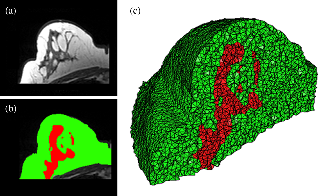

Fig. 5

Original CT slice of the mouse (a), segmentation of different tissue types (b), and the 3-D tetrahedral mesh for the mouse (c), showing the regions as different colors: red is general tissue, green indicates the brain, and yellow is the tumor.

Fig. 6

Time comparison of segmentation and mesh creation from pancreas CT between Nirfast and the commercial package Mimics.

The resulting 3-D tetrahedral meshes from both programs were then analyzed to assess element quality. Also analyzed was a new mesh optimization feature in Nirfast. This is an optional procedure that searches the mesh for poor-quality elements and attempts to fix them to improve quality, as defined below. It can take a significant amount of time for large mesh sizes, but can vastly increase the quality. In this case, optimization took 15 min. The meshes were made to have a similar number of nodes: 224,049 for the Mimics mesh, 224,445 for the Nirfast mesh, and 224,989 for the optimized Nirfast mesh. The metric used for quality criterion is the sine of minimum dihedral angle of each tetrahedron. Values close to zero would indicate an almost flat element. Such elements can cause loss of numerical accuracy as well as make the stiffness matrix in the FEM formulation ill-conditioned. The optimal value of this quality would be $\sin (70.52\mathrm{deg})=0.942$ for an equilateral tetrahedron; however the upper bound is 1.0. Figure 7 shows the quality histograms using Mimics, Nirfast, and mesh optimization in Nirfast. The minimum quality for each case respectively was 0.06, 0.12, and 0.65, with average quality values of 0.71, 0.73, and 0.77.

Fig. 7

Histograms comparing mesh element quality between the commercial package Mimics and the tools developed in Nirfast. Also shown is the quality histogram when using the mesh optimization feature in Nirfast. No subsequent postprocessing improvements were applied to the Mimics mesh (but are available in the 3-matic package).

Figure 8 shows the reconstruction results in the mouse head using the Mimics mesh and the Nirfast mesh, displaying fluorescence yield overlaid on the MR images. The recovered fluorescence yield for each region in both cases is reported in Table 4.

Fig. 8

Reconstructed fluorescence yield overlaid on sagittal MR images of the mouse head, based on reconstructions on a mesh created in Mimics (a) and in Nirfast (b). The fluorescence tomographic reconstructions are based on the segmentation of tissue types and region-based reconstruction on the resulting tetrahedral meshes.

Table 4

Recovered fluorescence yield for each region in reconstruction using the mouse head. Results are reported on both the Mimics- and Nirfast-created meshes.

4.

Discussion

New segmentation and mesh creation tools have been implemented in Nirfast, with the ability to work from the variety of medical images encountered in optical tomography. The efficacy of these tools has been compared with the commercial package Mimics in a case study. The minimum and average tetrahedron element quality values are better using Nirfast (especially when using mesh optimization). In particular, the minimum quality is 62% higher relative to the optimal value using Nirfast. Low-quality elements can produce erroneous numerical solutions by several orders of magnitude, or even prevent a solution from being computed, so this improvement in the minimum quality threshold is essential for DOT. There is a large difference in the amount of time spent, with Nirfast being far more efficient by approximately fivefold. In segmentation, this is partly affected by the efficiency of the automatic segmentation methods, and also by the availability of many advanced segmentation tools that are particularly useful for the typical contrast profiles seen in MR/CT. A good example is breast imaging using MR guidance, where low-frequency gradients are often seen in the images. In the past, this has often hindered the ability to segment these images, as grayscale values of the same tissue type will no longer be in the same range.⁴⁸ These gradients can be easily removed using MR bias removal, thus greatly reducing the amount of manual touch-up needed after automatic segmentation. In meshing, the improved computational time is in part due to the fact that the new meshing tools are completely automatic and do not require any fixing after mesh creation. The metrics used for speed and quality in comparison with Mimics account for all pre- and post-processing done using tools available in Mimics to improve mesh quality, but not any external tools that may be used separate from Mimics. For example, 3-matic is also a tool marketed by Materialise, capable of postprocessing mesh quality improvement, which could significantly improve the quality of meshes produced by Mimics.

An advantage of the Nirfast package that is not evident from the time benchmarks is the ease of use in the workflow. Since the entire package has been designed around seamlessly segmenting, creating a mesh, modeling light transport, and then visualizing the result, it is much easier to use than a combination of packages that are not optimized for optical tomography. In reconstruction results, as seen in Fig. 8, the recovered fluorescence yield is very similar between Mimics and Nirfast. In fact, there is a small improvement in the tumor and tumor boundary to background tissue fluorescence yield contrast recovered. This indicates that the new tools do not adversely affect reconstruction, despite saving significant time during segmentation and mesh creation. Furthermore, the higher minimum element qualities ensure that numerical issues do not arise with generating forward data on a poor-quality mesh, which can often cause a reconstruction to fail entirely and terminate before converging upon a solution.

The tools have been presented with a focus on optical tomography and the types of medical images often encountered in image-guided optical tomography. However, these tools could certainly be used for other applications in which it is useful to have a 3-D tetrahedral mesh created from 2-D image slices, such as electrical impedance tomography. One of the advantages of the meshing tools presented is the fact that interior region surfaces are maintained in the mesh, as opposed to simply labeling interior elements based on region proximity. This is very important in FEM modeling for optical tomography, as having the boundary of a surface inaccurately represented can lead to poor quantification.⁴⁹

5.

Conclusion

Tools have been created to allow for segmentation and 3-D tetrahedral mesh creation from a variety of medical images and systems used in optical tomography applications. These tools show promising computational time and element quality benchmarks. The ease and speed of segmentation and meshing is very useful in promoting the use of optical tomography, which has long suffered from long, difficult, and nonrobust meshing procedures. Furthermore, the available automatic segmentation modules provide essential tools for many different types of medical images, particularly in regard to artifacts often seen in MR images. The tools are provided as part of a complete package designed for modeling diffuse light transport in tissue, allowing for a seamless workflow that has never before been available.