1.

Introduction

Fluorescence diffuse optical tomography (fDOT) is an imaging modality that aims at reconstructing three-dimensional (3-D) distributions of fluorescent markers embedded within biological tissues.¹ This technology has facilitated monitoring of molecular activity, tumor growth, response to drug therapy, etc., mostly in small animals.

In fDOT, a near-infrared (NIR) light source at excitation wavelength is illuminated onto the subject under study at different positions. Fluorophores absorb the excitation light and re-emit part of the energy at a longer wavelength. In most modern noncontact fDOT systems, light intensity measurements (CW) at the emission, and possibly, excitation wavelengths are collected by a charged-coupled device (CCD) camera placed opposite to the light source, which is rotated around the object of study.²

The image reconstruction consists of the inversion of a linear operator (sensitivity matrix), mapping the fluorescence yield of the fluorophore, which is linearly related to its concentration, to the measured data. However, due to the diffusive nature of light propagation in biological tissue the image reconstruction is an ill-posed inverse problem, meaning that noise in the data may give rise to significant errors in the reconstructed image.

The ill-posedness of the problem can be reduced by using large data sets.^3,4 The use of CCD cameras produces large amounts of data, typically of the order of $n_{\mathrm{meas}}\sim {10}^7$. However, this makes the problem large scale and more challenging to solve. Furthermore, the parameters to reconstruct are so numerous, $n_{\mathrm{recon}}\sim {10}^6$, that the sensitivity matrix is extremely large. The large matrix size poses a problem for storage, as well as computation time required for inversion. Therefore, specialized algorithms that can handle problems with large dimensions are required.

Markel and Schotland^3,5 proposed a series of algorithms for the reconstruction of images from extremely large data sets, which exploit symmetry properties of simple geometries. Konecky et al.⁶ reconstructed diffuse optical tomography (DOT) images using a fast inversion method, which combines plane wave illumination⁷ with analytic image reconstruction methods. The reconstruction method exploits the block structure of the linear operator that couples the measurements to the optical properties of the object of study, and hence, instead of inverting a large matrix, the problem is reduced to inverting a set of relatively small matrix blocks. Lukic et al.⁸ used a similar method, but replaced point sources by structured illumination (Fourier encoding), and hence, data are directly measured in the Fourier space. Since DOT suffers from low spatial resolution, only a few low Fourier components retain relevant information. In this approach, the inverse problem is fully Fourier encoded, i.e., sources, detectors, and solution space are represented in the Fourier space. Ducros et al.⁹ used a similar approach, but based on wavelet encoding methods. Ripoll¹⁰ proposed a hybrid approach, where only the measurements are Fourier encoded, while the sources and solution space are kept in the real space. However, most of these approaches are based on analytical expressions (Green’s functions) for the slab geometry.

For complex geometries, an alternative is to use a matrix-free Krylov-subspace approach, in which the storage of the sensitivity matrix is replaced by vector-matrix products, i.e., solving the forward and adjoint problems where the solutions are computed numerically using the finite element method (FEM).¹¹ The matrix-free method relies on iterative Krylov-subspace methods, such as generalized minimal residual method, which may suffer from slow convergence. Therefore, the method overcomes the storage problems of large data sets at the expense of computational efficiency.

Multigrid methods offer the capability of reconstructing images at lower spatial scales by solving smaller instances of the problem, which allows approximate solutions to be computed quickly at low resolution and progressively refined. Zhu et al.¹² developed a wavelet-based multigrid approach. The rows and columns of the sensitivity matrix are wavelet transformed and the system at a coarser resolution is solved. Solutions at coarser resolutions are used as the initial guess for solving systems at finer resolutions. It is also possible to select regions of interest at smaller scales based on coarse level reconstructions. However, in order to maintain reconstruction resolution, this approach requires reconstructions at many scales, and thus, does not result in significant reduction in computation time. Furthermore, it requires the full sensitivity matrix to be calculated and stored.

Another approach is to use the wavelet-Galerkin method to generate the forward model, instead of using the more time consuming FEM (Ref. 13). However, unlike FEM, this method is only applicable to simple geometries, but the fictitious domain method is used to overcome this limitation.¹⁴ In the wavelet-Galerkin method, the wavelet scaling functions are used as a basis on a regular grid. This allows a more compact representation of the problem and the use of multigrid techniques. As before, solutions can be obtained at progressively higher wavelet resolution scales, terminating when appropriate. Although this is an efficient way to compute the full matrix for large solution spaces, it is not suitable for large data sets.

Wavelets were also used in Ref. 15 to reduce the fDOT forward model computation time by projecting the original FEM matrices into a series of wavelet bases.

This paper proposes a method that reduces significantly the size of the sensitivity matrix by compressing its rows and columns using wavelets, allowing it to be stored explicitly while maintaining the spatial resolution and accuracy of the reconstructed images and low-computational time. This method is an extension of the work in Ref. 16, where wavelet compression is applied to a very large data sets in order to reduce data space dimensions. Here, a similar approach is used to reduce the solution space dimensions. Therefore, given the reduced dimensions of the image reconstruction problem, the solution can be found using direct inversion methods. The performance of the method is assessed using simulations and experimental phantom data. The effect of incorporating a priori structural information into the compressed image reconstruction is also analyzed.

2.

Methods

2.3.

Fast Wavelet Transform

The fast wavelet transform (FWT) decomposes a signal or function $f_0$ into different frequency subbands.²² It uses a low-pass filter $h$ and a high-pass filter $g$ to obtain the approximation Wc and detail Wd coefficients. The approximation coefficients represent the approximation of the signal at a resolution $2^j$, where $j$ is an integer that specifies the resolution level. The detail coefficients contain the details of the original signal, i.e., the high-frequency information. For a signal $f(n)=\mathbf{W}(j+1,n)$, with $n$ samples and at a starting scale $j+1$

Eq. (16)

$$\mathrm{Wc}(j,n)=h(-n)*\mathrm{Wc}(j+1,n)\downarrow 2,$$

Eq. (17)

$$\mathrm{Wd}(j,n)=g(-n)*\mathrm{Wd}(j+1,n)\downarrow 2.$$

Thus, the FWT consists of a convolution, followed by downsampling by a factor of 2 ($\downarrow 2$), i.e., keeping the even index samples. The wavelet transform can be implemented as a decomposition filter bank, where the initial signal goes through a series of filters. The synthesis filter bank can be used to perform the inverse transform (IFWT) and reconstruct the signal $f_0$. First, the signal is upsampled by a factor of 2 ($\uparrow 2$), i.e., adding a zero between samples, followed by convolution with the inverse filter. Note that the filters are related to each other by $g(n)={(-1)}^{n}h(1-n)$. Figure 1 shows a one-level decomposition and synthesis filter bank.

Fig. 1

One-level 1-D FWT and IFWT.

The separability property of the two-dimensional (2-D) wavelet transform means that performing a 2-D wavelet transform is equivalent to performing two one-dimensional (1-D) transforms, i.e., one 1-D transform along with the columns of the image $f(m,n)$ ($n$-axis) and another 1-D transform along with the rows of $f(m,n)$ ($m$-axis) (Fig. 2). Analogously, performing a 3-D wavelet transform is equivalent to performing three 1-D transforms. The same applies to the IFWD in higher dimensions.

Fig. 2

One-level 2-D FWT.

2.3.1.

Data compression

Data compression is used to reduce the dimensions of the data for computational efficiency,¹⁶ while simultaneously reducing the redundancy of the data. We apply a four-level 2-D FWT (${\mathcal{W}}_{2\text{-}\mathrm{D}}$) to the projection image ${\mathbf{y}}_i^{e,f}$ captured by a CCD camera, where $i=1,2,\dots ,M_s$. The obtained wavelet coefficients are $W=\{\mathrm{Wc}(j-3,x,y),\mathrm{Wd}1(j-k,x,y),\mathrm{Wd}2(j-k,x,y),\mathrm{Wd}3(j-k,x,y):j=7\text{and}0\le k\le 3\}$, where Wd1, Wd2, and Wd3 are the detail coefficients that passed through a high-pass filter at least once. We keep the coefficients that are larger than a threshold $T_M$, set to the $M_{\psi }$ largest coefficients (i.e., $M_{\psi }=W>T_M$), which contain most of the relevant information, and hence, the dimensions of the vectorized compressed data $\tilde{\mathbf{y}}$ are reduced to $M_s\times M_{\psi }$. For example, if $W_T=128\times 128$ is the total number of wavelet coefficients, then $T_M=W_{\mathrm{sort}}(P\times W_T)$, where $W_{\mathrm{sort}}$ are the wavelet coefficients sorted in descending order and $P$ is the percentage of coefficients to be removed. If $P=0.98$, then $M_{\psi }=328$ and the compressed data $\tilde{\mathbf{y}}$ has dimensions $18\times 328$. Similarly, the size of the row compressed Jacobian $\tilde{J}$ is reduced to $(M_s\times M_{\psi })\times N$. The resulting compressed forward problem is $\tilde{\mathbf{y}}=\tilde{J}\tilde{\mathbf{f}}$.

2.3.2.

Solution compression

In this paper, we extend the work in Ref. 16 by applying a similar wavelet compression to each row of the Jacobian, thus reducing the dimensions of the solution space. Each row $r_i$ of the Jacobian represents the sensitivity of one measurement $\widehat{\mathbf{y}}$ (matrix $J$) or compressed measurement $\tilde{\mathbf{y}}$ (matrix $\tilde{J}$) to changes in $f$. Both $f$ and $r_i$ represent 3-D images of dimensions $N_x\times N_y\times N_z$, and therefore, a 3-D FWT (${\mathcal{W}}_{3\text{-}\mathrm{D}}$) is performed on the rows of the sensitivity matrix. Two methods are investigated, one where the sensitivity matrix is sparse and another where the matrix is fully compressed.

Sparse matrix: A highly sparse matrix $\breve{J}$ can be obtained by keeping the wavelet coefficients $V$ larger than a threshold $T_N$, set to the $N_{\mathrm{\Psi }}^{\mathrm{th}}$ largest coefficient in each row, and setting the remaining coefficients to zero

Eq. (18)

$${\breve{J}}_{ij}=\{\begin{array}{cc}{V}_{ij},& \text{if}{V}_{ij}>T_N\\ 0,& \text{elsewhere}\end{array},$$

where the subscript $i$ is the row index and $j$ is the column index. For example, if $W_{\mathrm{T}2}=64\times 64\times 64$ is the total number of wavelet coefficients, then $T_N=V_{\mathrm{sort}}(P\times W_{\mathrm{T}2})$, where $V_{\mathrm{sort}}$ are the wavelet coefficients sorted in descending order. If we consider $P=0.98$, then $N_{\mathrm{\Psi }}=5243$.

The resulting forward problem, using data and solution compression, is $\tilde{\mathbf{y}}=\text{sparse}(\breve{J})\breve{\mathbf{f}}$. The solution is a sparse image of size $N_x\times N_y\times N_z$ and $N_{\mathrm{\Psi }}$ nonzero elements. The matrix $\breve{J}$ has dimensions $(M_s\times M_{\psi })\times (N_x\times N_y\times N_z)$ and $(M_s\times M_{\psi })\times N_{\mathrm{\Psi }}$ nonzero elements. The solution is obtained by solving the inverse problem and performing a 3-D IFWT (${\mathcal{W}}_{3\text{-}\mathrm{D}}^{-1}$) to $\breve{\mathbf{f}}$.

Fully compressed matrix: Alternatively, if only $N_{\mathrm{\Psi }}$ wavelet coefficients are kept, then the size of the compressed Jacobian $\overline{J}$ is reduced to $(M_s\times M_{\psi })\times N_{\mathrm{\psi }}$. The forward problem is $\tilde{\mathbf{y}}=(\overline{J})\overline{\mathbf{f}}$, where $\overline{\mathbf{f}}$ is a vector of size $N_{\mathrm{\Psi }}$. Therefore, the solution is a compressed image of size $N_{\mathrm{\Psi }}$, which is converted into a sparse $N_x\times N_y\times N_z$ image and inversely wavelet transformed. Consider $A_i={\mathcal{W}}_{3\text{-}\mathrm{D}}\{r_i\}$ and $A_M=\text{mean}(A_i)$ (average along the rows), the wavelet coefficients kept correspond to the $j_N$ location of the $N_{\mathrm{\Psi }}^{\mathrm{th}}$ largest $A_M$ elements: ${\overline{J}}_{i,j}=A_{i,j_N}$. Unlike the sparse matrix method, where the $j_N$ location corresponds to the location of the $N_{\mathrm{\Psi }}^{\mathrm{th}}$ largest coefficients in each row and, therefore, the $j_N$ locations are different for each row, in the fully compressed method the $j_N$ locations are the same in all the rows of the wavelet transformed matrix $A$.

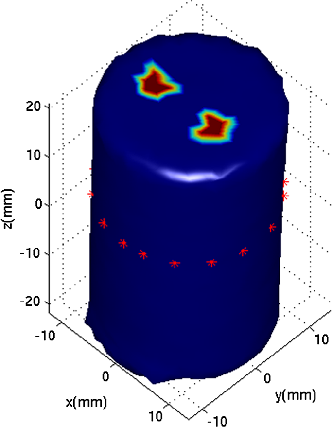
2.5.

Evaluation

The performance of our data and solution compression method is evaluated through simulations and a phantom study. The matrix $J$ is calculated using TOAST, which is an FEM based software developed at University College London (UCL). Images are reconstructed (a) using zero-order Tikhonov regularization and solving the linear problem directly and (b) iteratively using our ADSP method.²⁰ Solutions are computed on a tetrahedral mesh and mapped into a regular $64\times 64\times 64$ grid covering the domain of the mesh.

In the following sections, we refer to the data compression method as DC, sparse matrix method as $S_x$ and the fully compressed matrix method as ${\mathrm{FC}}_x$, where $x$ represents the number of coefficients $N_{\mathrm{\Psi }}$.

Wavelet filters: After experimenting different wavelet filters, we choose to use the Battle–Lemarié wavelet filters, which appear to be suitable for this type of application. The Battle–Lemarié wavelets are symmetric, orthonormal, and smooth. These wavelets are attractive since they have good time and frequency localization properties and can approximate smooth solutions.²² Other popular wavelets, such Daubechies, are not smooth enough and do not possess good frequency localization.²³

Battle–Lemarié wavelet filters are built from polynomial splines of order $2p+1$. Let $\varphi (\omega )$ be the Fourier transform of the wavelet scaling function $\varphi (t)$. The low-pass quadrature mirror filter $H(\omega )$ can be obtained from the following relation in the Fourier domain²²

Eq. (19)

$$\varphi (2\omega )=H(\omega )\varphi (\omega ),\text{where}H(\omega )\sum _{n=-\infty }^{\infty }h(n)e^{-in\omega }.$$

Lemarié has shown that the scaling function can be written as

Eq. (20)

$$\varphi (\omega )=\frac{1}{{\omega }^n\sqrt{{\mathrm{\Sigma }}_{2n}(\omega )}},\text{where}n=2+2p,$$

and where

Eq. (21)

$${\mathrm{\Sigma }}_n(\omega )=\sum _{k=-\infty }^{\infty }\frac{1}{{(\omega +2k\pi )}^n}.$$

Alternatively, one can calculate ${\mathrm{\Sigma }}_n(\omega )$ by computing the $n-2$ derivative of the formula:

Eq. (22)

$${\mathrm{\Sigma }}_2(\omega )=\frac{1}{4{\sin }^2(\omega /2)}.$$

For an approximation built from cubic splines, i.e., $p=1$, and thus, $n=4$, it follows from the previous equations that

Eq. (23)

$$\varphi (\omega )=\frac{1}{{\omega }^4\sqrt{{\mathrm{\Sigma }}_8(\omega )}}\mathrm{and}H(\omega )=\sqrt{\frac{{\mathrm{\Sigma }}_8(\omega )}{2^8{\mathrm{\Sigma }}_8(2\omega )}}.$$

Figures of merit: The relative error (RE) and contrast-to-noise ratio (CNR) are used to evaluate the quality of the reconstructed images. The RE between the true image $f_{\text{true}}$ and the reconstructed image $f_{\mathrm{recon}}$ is defined as $\mathrm{RE}={\parallel f_{\text{true}}-f_{\mathrm{recon}}\parallel }_2/{\parallel f_{\text{true}}\parallel }_2$. The CNR is calculated as follows:²⁴

Eq. (24)

$$\mathrm{CNR}=\frac{{\mu }_{\mathrm{ROI}}-{\mu }_{\mathrm{B}}}{{[w_{\mathrm{ROI}}{\sigma }_{\mathrm{ROI}}^2-w_{\mathrm{B}}{\sigma }_{\mathrm{B}}^2]}^{1/2}},$$

where ${\mu }_{\mathrm{ROI}}$ is the mean value of the region of interest (ROI); ${\mu }_{\mathrm{B}}$ is the mean value of the background (B); ${\sigma }_{\mathrm{ROI}}$ and ${\sigma }_{\mathrm{B}}$ are the standard deviations of the ROI and background, respectively; and $w_{\mathrm{ROI}}=A_{\mathrm{ROI}}/(A_{\mathrm{ROI}}+A_{\mathrm{B}})$ and $w_{\mathrm{B}}=A_{\mathrm{B}}/(A_{\mathrm{ROI}}+{\text{Area}}_{\mathrm{B}})$ are noise weights, where $A_{\mathrm{ROI}}$ and $A_{\mathrm{B}}$ are the ROI and B areas, respectively. The ROI is defined as the region where voxels have attained at least half maximum intensity and the remaining voxels represent the background B.

2.5.1.

Simulation

The geometry used in the simulation is similar to the phantom geometry. The matlab package Iso2mesh²⁵ was used to generate a tetrahedral mesh from the X-ray computed tomography (XCT) image of a cylindrical phantom (see Sec. 2.5.2 and Fig. 3). The FEM mesh has 8449 nodes, 49,797 elements and dimensions $28\times 28\times 42{\mathrm{mm}}^3$. Similar to the phantom, the optical properties are ${\mu }_a=0.01{\mathrm{mm}}^{-1}$ and ${\mu }_s^{\prime }=0.8{\mathrm{mm}}^{-1}$, and the fluorescent targets are two vertical cylinders placed parallel to each other (Fig. 3) with contrast $f=2$. Projection images of size $128\times 128$ pixels are calculated for 18 evenly spaced source-camera positions over a full 360 degrees range at $z=0\mathrm{mm}$ (Fig. 3). Data consist of fluorescence and excitation projections with 2% Gaussian random noise. The data space is compressed by setting $M_{\psi }=32$ and solutions are computed with $N_{\mathrm{\Psi }}=\{\mathrm{8192,4096,1024,256}\}$. For the reconstructions using zero-order Tikhonov regularization the damping factor is initially set to ${\lambda }_{\mathrm{Tik}}=a\text{trace}(J_c{J}_c^T)$ and for reconstructions using ADSP regularization it is set to ${\lambda }_{\mathrm{ADSP}}=10a\text{trace}(J_c{J}_c^T)$, where $a=3\times {10}^{-4}$ and $J_c$ are the different types of compressed Jacobian matrices.

Fig. 3

Geometry used in the simulations. The FEM mesh is generated from X-ray CT images of the experimental phantom. The asterisk markers indicate the source positions.

2.5.2.

Phantom

Data are acquired using the rotating fDOT–XCT system described in Ref. 2. The optical and XCT images are acquired sequentially. The solid phantom consists of a mixture of Agar, Intralipid, and ink. The stock solution is 4.56 ml Intralipid 20% (Sigma–Aldrich Co. LLC, St. Louis, USA), 0.256 ml India ink, 100 ml deionized water and 2.8 g Agar (Sigma–Aldrich Co. LLC, St. Louis, USA). The phantom is a cylinder with diameter $\varnothing =28\mathrm{mm}$, height $L=65\mathrm{mm}$ and optical properties ${\mu }_a=0.01{\mathrm{mm}}^{-1}$ and ${\mu }_s^{\prime }=0.8{\mathrm{mm}}^{-1}$, which were measured using a spectrometer (USB4000-VIS-NIR, Ocean Optics, London, UK). Two translucent tubes with an inside diameter of 3 mm (and outside diameter 4 mm) are inserted parallel to its long axis and filled with an optically matched fluid containing a fluorescent dye (Alexa 750) at 500 nM (molar) concentration. Excitation and fluorescence data images of size $512\times 512$ (resized to $128\times 128$) are recorded at 18 angular positions (same than the simulations). The FEM mesh is the same than the one used in the simulation study. We use the compression $M_{\psi }=32$ and $N_{\mathrm{\Psi }}=\{\mathrm{1024,256}\}$ ($N_{\mathrm{\Psi }}=256$ when ADSP regularization is used). The damping factor is initially set to ${\lambda }_{\mathrm{Tik}}=a\text{trace}(J_c{J}_c^T)$ and ${\lambda }_{\mathrm{ADSP}}=10a\text{trace}(J_c{J}_c^T)$, where $a=8\times {10}^{-3}$.

3.

Results

Profile plots across the reconstructed fluorescence targets ($z=0\mathrm{mm}$ and $y=0\mathrm{mm}$) are shown in Figs. 4 and 5 for images obtained using Tikhonov regularization for the sparse and fully compressed matrix cases, respectively. Similarly, Figs. 6 and 7 show the profile plots for images obtained using ADSP regularization. Figures 4 and 6 also show the profile plots for the data compression case.

Fig. 4

Profile plots across the fluorescence images ($z=0\mathrm{mm}$ and $y=0\mathrm{mm}$) reconstructed from simulated data using Tikhonov regularization and data compression, a sparse matrix with different compression levels, and the true solution.

Fig. 5

Profile plots across the fluorescence images ($z=0\mathrm{mm}$ and $y=0\mathrm{mm}$) reconstructed from simulated data using Tikhonov regularization and a fully compressed matrix with different compression levels, and the true solution.

Fig. 6

Profile plots across the fluorescence images ($z=0\mathrm{mm}$ and $y=0\mathrm{mm}$) reconstructed from simulated data using ADSP regularization and data compression, a sparse matrix with different compression levels, and the true solution.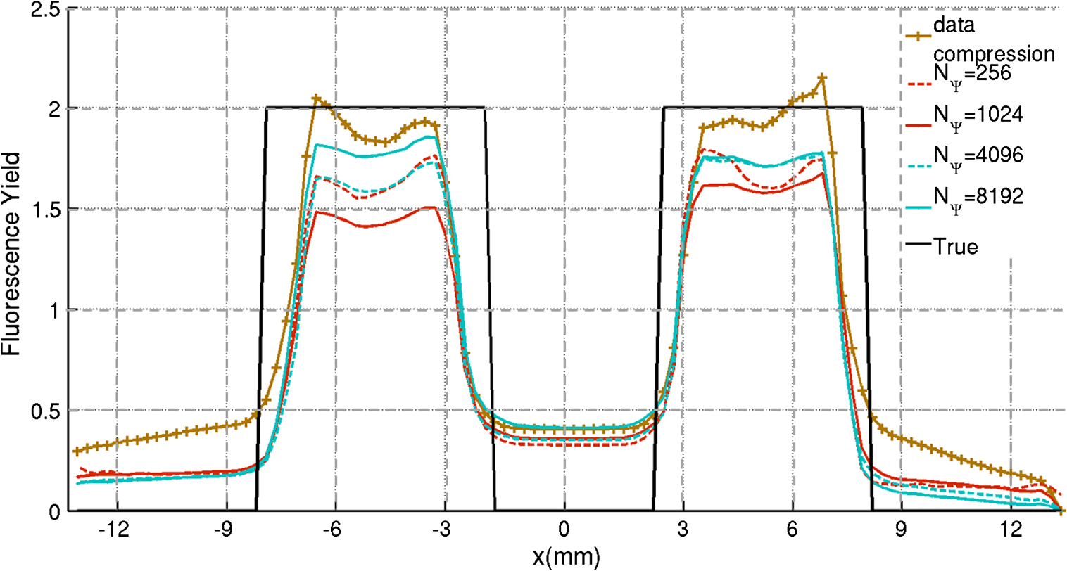

Fig. 7

Profile plots across the fluorescence images ($z=0\mathrm{mm}$ and $y=0\mathrm{mm}$) reconstructed from simulated data using ADSP regularization and a fully compressed matrix with different compression levels, and the true solution.

Since the profiles across the fluorescent inclusions do not differ significantly for the different types of compression, particularly when ADSP regularization is used, only results obtained without solution compression and high levels of solution compressions are shown. Therefore, reconstructions obtained using ADSP are shown for data compression and solution compression with $N_{\mathrm{\Psi }}=256$. Reconstructions obtained using Tikhonov regularization and solution compression with $N_{\mathrm{\Psi }}=\{\mathrm{1024,256}\}$ are displayed for comparison with the case where only data compression is used, to show the effect of the solution compression on the noise in the reconstructions.

The fluorescence distribution images reconstructed from simulated data using zero-order Tikhonov regularization are shown in Figs. 8Fig. 9Fig. 10Fig. 11–12. The reconstructions are displayed as 3-D isosurfaces (70% of the maximum value) together with the structural volumetric image. Additionally, a 2-D cross section of the reconstructed volume is taken at $z=0\mathrm{mm}$ and thresholded at 70% of the maximum value. The thresholded images are overlaid onto the structural image. Figures 13Fig. 14–15 show the images reconstructed using ADSP regularization and thresholded at 50% of the maximum value. The threshold value is lower since these images are not as contaminated with noise as the previous ones.

Fig. 8

Fluorescence yield $f$ reconstructed from simulated data using Tikhonov regularization and data compression in (left) 3-D and (right) 2-D cross section at $z=0\mathrm{mm}$.

Fig. 9

Fluorescence yield $f$ reconstructed from simulated data using Tikhonov regularization and $S_{1024}$ in (left) 3-D and (right) 2-D cross section at 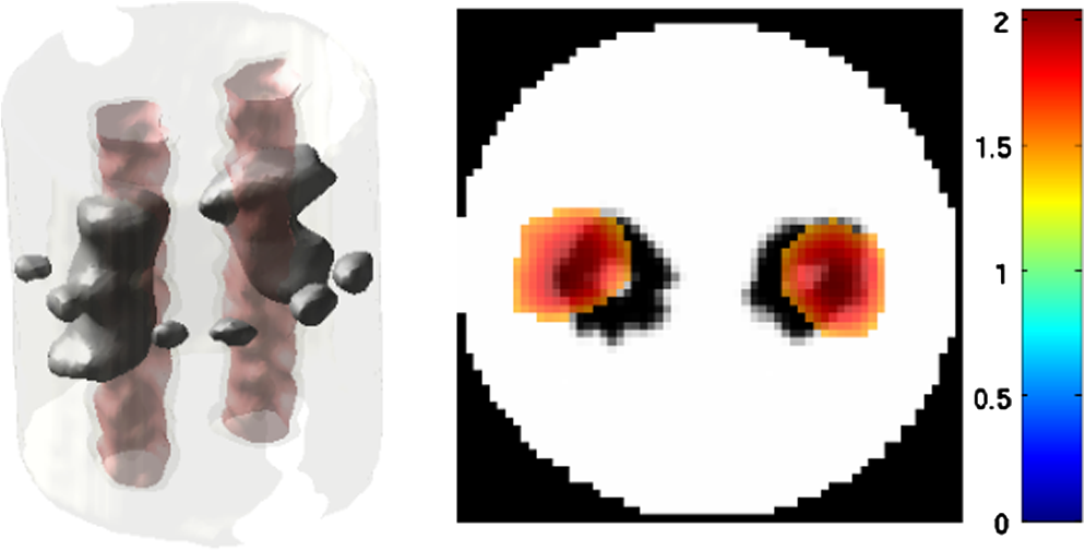$z=0\mathrm{mm}$.

Fig. 10

Fluorescence yield $f$ reconstructed from simulated data using Tikhonov regularization and $S_{256}$ in (left) 3-D and (right) 2-D cross section at $z=0\mathrm{mm}$.

Fig. 11

Fluorescence yield $f$ reconstructed from simulated data using Tikhonov regularization and ${\mathrm{FC}}_{1024}$ in (left) 3-D and (right) 2-D cross section at $z=0\mathrm{mm}$.

Fig. 12

Fluorescence yield $f$ reconstructed from simulated data using Tikhonov regularization and ${\mathrm{FC}}_{256}$ in (left) 3-D and (right) 2-D cross section at $z=0\mathrm{mm}$.

Fig. 13

Fluorescence yield $f$ reconstructed from simulated data using ADSP regularization and data compression in (left) 3-D and (right) 2-D cross section at $z=0\mathrm{mm}$.

Fig. 14

Fluorescence yield $f$ reconstructed from simulated data using ADSP regularization and $S_{256}$ in (left) 3-D and (right) 2-D cross section at 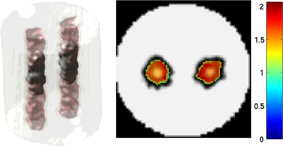$z=0\mathrm{mm}$.

Fig. 15

Fluorescence yield $f$ reconstructed from simulated data using ADSP regularization and ${\mathrm{FC}}_{256}$ (left) 3-D and (right) 2-D cross section at $z=0\mathrm{mm}$.

Similarly, the images reconstructed from phantom data using zero-order Tikhonov regularization are shown in Figs. 16Fig. 17Fig. 18Fig. 19–20 and using ADSP regularization are shown in Figs. 21Fig. 22–23. Their respective profile plots are shown in Figs. 24 and 25.

Fig. 16

Fluorophore concentration (nM) reconstructed from phantom data using Tikhonov regularization and data compression in (left) 3-D and (right) 2-D cross section at 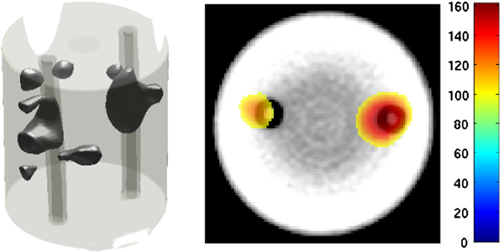$z=0\mathrm{mm}$.

Fig. 17

Fluorophore concentration (nM) reconstructed from phantom data using Tikhonov regularization and $S_{1024}$ in (left) 3-D and (right) 2-D cross section at $z=0\mathrm{mm}$.

Fig. 18

Fluorophore concentration (nM) reconstructed from phantom data using Tikhonov regularization and $S_{256}$ in (left) 3-D and (right) 2-D cross section at 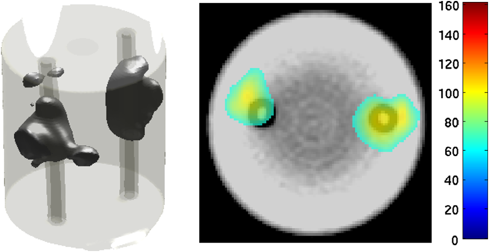$z=0\mathrm{mm}$.

Fig. 19

Fluorophore concentration (nM) reconstructed from phantom data using Tikhonov regularization and ${\mathrm{FC}}_{1024}$ in (left) 3-D and (right) 2-D cross section at $z=0\mathrm{mm}$.

Fig. 20

Fluorophore concentration (nM) reconstructed from phantom data using Tikhonov regularization and ${\mathrm{FC}}_{256}$ in (left) 3-D and (right) 2-D cross section at $z=0\mathrm{mm}$.

Fig. 21

Fluorophore concentration (nM) reconstructed from phantom data using ADSP regularization and data compression in (left) 3-D and (right) 2-D cross section at $z=0\mathrm{mm}$.

Fig. 22

Fluorophore concentration (nM) reconstructed from phantom data using ADSP regularization and $S_{256}$ in (left) 3-D and (right) 2-D cross section at $z=0\mathrm{mm}$.

Fig. 23

Fluorophore concentration (nM) reconstructed from phantom data using ADSP regularization and ${\mathrm{FC}}_{256}$ in (left) 3-D and (right) 2-D cross section at $z=0\mathrm{mm}$.

Fig. 24

Profile plots across the fluorescence images ($z=0\mathrm{mm}$ and $y=0\mathrm{mm}$) reconstructed from phantom data using Tikhonov regularization and DC, $S_{256}$, ${\mathrm{FC}}_{256}$, and the true solution.

Fig. 25

Profile plots across the fluorescence images ($z=0\mathrm{mm}$ and $y=0\mathrm{mm}$) reconstructed from phantom data using ADSP regularization and DC, $S_{256}$, ${\mathrm{FC}}_{256}$, and the true solution.

Figures 26 and 27 show the RE and CNR, respectively, of the images reconstructed from simulated and phantom data using Tikhonov and ADSP regularization for the different compression methods. Figure 28 shows the condition number of the matrices in the data compression, compressed sparse, and fully compressed format.

Fig. 26

RE of images reconstructed from (left column) simulated data and (right column) phantom data using (top row) Tikhonov regularization and (bottom row) ADSP regularization, for the different compression cases.

Fig. 27

CNR of images reconstructed from (left column) simulated data and (right column) phantom data using (top row) Tikhonov regularization and (bottom row) ADSP regularization, for the different compression cases.

Fig. 28

Condition number of the data compressed, sparse, and fully compressed matrices.

The reconstructions are faster when a fully compressed matrix is used, and the sparse matrix method is faster than using data compression only, with a ratio of $9.3:3.9:1$.

4.

Discussion and Conclusion

In fDOT, the data and solution spaces can be quite large, and hence, the sensitivity matrix may be too large to store. Even if this matrix can be stored, it may not be possible to directly invert it, and thus, iterative methods must be employed. However, these are computationally expensive and may take a long time to converge. The method we proposed reduces the dimensions of the sensitivity matrix allowing the storage and direct inversion of the matrix and, for the sparse matrix case, without requiring the construction of the full matrix. Both sparse and fully compressed matrix representations allow storage of large amounts of data generated from CCD-based fDOT systems, rather than keeping redundant data and solution components.

The performance of our method was tested on simulated and experimental phantom data. Our simulations show that our solution compression approach can help to suppress noise in the reconstructed images (Figs. 8Fig. 9Fig. 10Fig. 11–12). This result is not surprising, since wavelet transforms are a common and efficient technique for denoising. The use of structural a priori information in the image reconstruction greatly improved the quality of the images (Figs. 6, 7, and 13Fig. 14–15). The images reconstructed using the different types of compression are qualitatively very similar. However, the fluorescence yield was underestimated when both data and solution compression were used with ADSP regularization. The images reconstructed from experimental data are similar (Figs. 16Fig. 17Fig. 18Fig. 19–20). The target locations and dimensions were accurately estimated by all the methods when structural information was incorporated into the image reconstruction (Figs. 21Fig. 22–23). The profiles plots in Figs. 24 and 25 also show that the use of structural information can greatly improve the quality of the reconstructions.

Our results show that the sensitivity matrix can be effectively compressed into a wavelet space by selecting the most significant wavelet coefficients. The sensitivity matrix, which in our studies has dimensions $576\times \mathrm{262,144}$, can effectively be represented in a fully compressed form with dimension $576\times 256$ or sparse form with size $576\times \mathrm{262,144}$ and $576\times 256$ nonzero elements.

Figure 26 shows that the RE decreases with increasing level of compression, i.e., the quality of the reconstruction improves, which is presumably a consequence of the decrease of the condition number (Fig. 28). The fully compressed matrix with $N_{\mathrm{\Psi }}=1024$ has a higher condition number, and hence, one should expect a higher RE. Nevertheless, the denoising characteristic of the wavelets seems to compensate for this effect. Figure 27 shows that the CNR of the images reconstructed from simulated data improves when solution compression is used, whereas the CNR of the images obtained from phantom data decreases. Overall, the simulation results using Tikhonov regularization with data and solution compression are quite similar, but the lowest RE was achieved with the ${\mathrm{FC}}_{256}$ method and the highest CNR using ${\mathrm{FC}}_{1024}$. For the phantom study, the best results were obtained with the ${\mathrm{FC}}_{256}$. The images reconstructed using ADSP and $S_{256}$ had the lowest RE and highest CNR.

The sparse matrix compression method has the advantage that the problem becomes less ill-conditioned and it does not require the explicit construction of the full matrix. The fully compressed matrix method provides images that are visually quite similar, but it underestimates the fluorescence yield more than the latter when ADSP is included. This method requires the construction of the full matrix and the wavelet coefficients kept in the compressed form are all in the same $j_N$ locations in all the rows of the matrix. These are not necessarily the most relevant coefficients, which may explain the lower qualitative accuracy. Nevertheless, this method allows a faster inversion process and, when Tikhonov regularization is used, provides images with the lowest RE and highest CNR.

The disadvantage of using ADSP regularization is that the solution depends on the parameter $\lambda$ value and the number of iterations until convergence is reached, i.e., it depends on the convergence criteria, and thus, there is still potential for improvement. Nevertheless, the results obtained using data and sparse matrix compression are quite satisfactory.

In this work, we map from the FEM mesh to a regular grid, which is then transformed into the wavelet space, with no regard to the irregular boundary of the object. In future work, we will attempt to apply a similar compression directly on the FEM mesh, so that the reconstruction is performed on the mesh and to avoid error propagation resulting from these mappings. Furthermore, the boundary of the object introduces sharp edges in the images, which may lead to artifacts in the compressed representation.

There is a large diversity of available wavelet filters, and hence, we performed a simple qualitative comparison of the suitability of some of the most popular ones (e.g., Haar, Daubechies, Coiflet, Symmlets, Battle–Lemarié, etc.) for use in fDOT. However, improved results can be expected if wavelet filters more adequate for the fDOT problem are designed and the ideal number of wavelet coefficients to keep is identified.

In summary, image reconstruction using data and solution compression can greatly reduce the dimensions and ill-conditioning of the problem, allowing fast and less noisy reconstructions.