|
|
1.IntroductionOral cancer is the sixth most common cancer among men in the world.1 Nowadays, in the developing countries, a higher rate of oral cancer incidence is observed in younger people, presumably due to the increased use of tobacco products. Though the five-year mortality rate of 42% and high morbidity rate are lower when compared with cervical, breast, and colorectal cancers,2–8 oral cancer is among leading cause of cancer-related deaths in the male population.9 In India, 320,000 new cancer cases are diagnosed annually in males, and 19% of this is oral cancer; in females out of 350,000 new cancer cases, 7% is oral cancer.10 Annually 640,000 oral cancer cases are diagnosed worldwide.11 In India, oral cancer stands in third position after breast and cervical cancers.10 One third of the world’s oral cancer cases are reported in India.12 Incidence of oral cancer is greater in males compared to females with a ratio of .11,13–15 A morphologically altered tissue, where cancer is more prone to occur than the normal, is considered as a precancerous lesion.16 Leukoplakia, erythroplakia, oral submucous fibrosis (OSMF), and lichen planus are the main oral precancerous lesions. The malignant transformation of leukoplakia, erythroplakia, and OSMF is well described at present.17,18 Leukoplakia is reported to have a malignant transformation rate from 0.13% to 19.8%.19–22 Erythroplakia is said to have more than 50% malignant transformation rate.23–27 Only the erosive form of lichen planus has a potential to turn into malignant form with a transformation rate of below 1%.25 The risk of malignant transformation of dysplasia ranges from 10% to 14%.28 Malignant transformation rate of 4.5% to 7.6% was reported for OSMF.29 Areca nut chewing is reported to be the causative agent for OSMF.29 In spite of the easy accessibility of the oral cavity, in the majority of cases the disease is detected only in the advanced stages contributing to higher morbidity and mortality rates. Early detection of the cancer is the most effective means of controlling the death rate and the cost of treatment.30 The failure in early detection by dentists and physicians is attributed to the fact that “physicians do not routinely inspect their patients for suspicious oral lesions, and dentists are also remiss in the early diagnosis and referral for oral cancer.”31 We have shown in our earlier work that pattern analysis of protein profiles of saliva, serum,32–35 and other clinical samples36–39 may provide a sensitive method for early detection of oral (and other) premalignant and malignant conditions. The suggestion that “multiparametric biomarker analysis with artificial neural networks and pattern recognition will likely represent one of the promising methodologies for diagnosing and monitoring cancer” has also been made by other workers.40 Recently, other groups also have proposed the use of markers in saliva41–43 for possible early diagnosis of different forms of malignancies. It is now established41 that more than 1000 proteins are present in saliva, and the level of many of them changes42 in malignancy. In addition, many salivary proteins are degraded under normal conditions of handling, storage, processing, etc., and these reactions themselves can be different under normal and disease conditions due to presence of altered enzymes and reactive proteins. The changes originally arising from disease conditions as well as those taking place after procurement have to be properly identified and quantified for diagnostic applications. Minimally invasive, inexpensive collection, simple handling and transportation, storage, and no risk in sampling make saliva an ideal biofluid for disease diagnosis.44–46 The simple collection method reduces the anxiety and discomfort, thereby making it user friendly for patients. Scientists often call saliva the “mirror of the body” and the “window on health status”.46 In view of the serious limitations of present oral cancer diagnostic methods,47 it is thus very essential to establish the feasibility of the use of saliva for early diagnosis of oral (or any other) malignancy, and to standardize procedures for protein profile analysis of saliva samples for early detection of oral cancer. In the present work we have used our method of High-performance liquid chromatography-laser-induced fluorescence (HPLC-LIF) protein profile analysis of saliva to systematically investigate the suitability of the technique for early detection of oral premalignancy and malignancy. 2.Methods and MaterialsWhole unstimulated saliva was collected from a group of 37 healthy, 40 premalignant, and 23 malignant subjects (sample information given in Table 1). The 40 premalignant subjects consist of 15 oral leukoplakia, 19 OSMF, and 6 oral lichen planus cases. The patients’ age groups were: premalignant 23 to 58 years and malignant 25 to 75 years. Ethical clearance for the current study has been obtained from the Kasturba Medical College, Manipal University Ethical Committee. Samples were collected with informed consent. Samples were collected after clinical/pathological diagnosis from the Department of Oral Medicine and Radiology, Manipal College of Dental Sciences, Mangalore. The clinical/pathological results of validation set samples (blind) were conveyed to the protein profile analysis group only after their data processing and diagnosis of test samples. Classification of samples was done by comparing with a control group of 37 healthy subjects from both genders (age range of 20 to 36 years) with no oral or systemic diseases. Only one malignant and two premalignant patients had no history of smoking, tobacco chewing, or alcohol intake. Table 1Sample information.
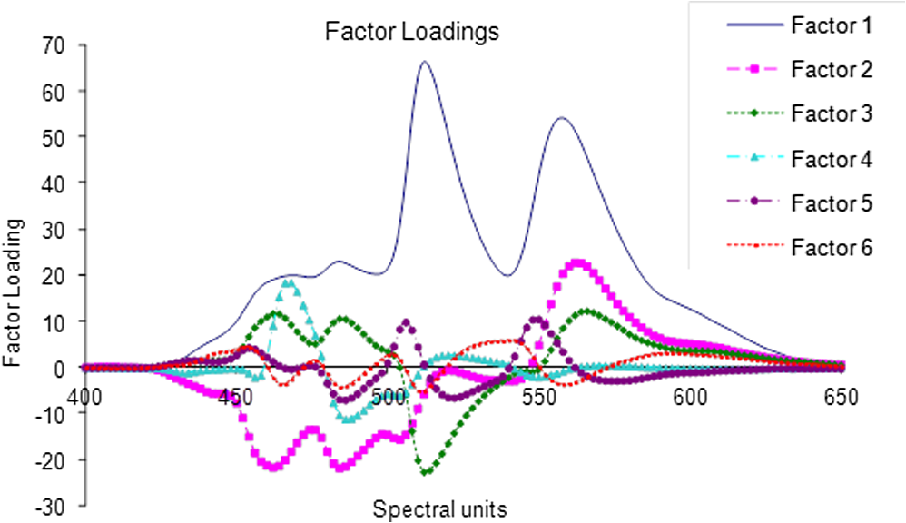
2.1.Sample Collection, Processing, and StorageWhole saliva was collected from the subjects after clinical examination. Subject’s mouth was cleaned with distilled water prior to sample collection. Volunteers were asked to generate saliva and spit into a wide mouth sterile sample collection bottle for about 5 to 10 min. Approximately 3 to 5 ml of whole saliva was collected from subjects. Bottles were immediately kept in ice buckets. Samples were transferred immediately to Eppendorf tubes and centrifuged twice at 5000 rpm for 10 min to remove any debris released in spite of the cleaning and also to eliminate exfoliated cells from the sample. Though exfoliated cells are useful in the diagnosis of malignancy,48 the major aim of the present studies was to identify “true” changes in salivary proteins in premalignant and malignant states. More importantly, it is well known49 that in early stages of malignancy/dysplasia, proliferation is confined to the basal layer. The cells move outward slowly to get sloughed off from the surface mostly only in advanced stages. The protein profiles of exfoliated cells that may appear randomly in any early stage may thus be not very useful for early detection and diagnosis. In the present studies, therefore, only the supernatant after centrifugation was collected and used. The supernatant was distributed into 3 to 5 aliquots, stored at for short-term storage, and used as soon as the system was ready for the next run. 2.2.Experimental SetupHPLC-LIF Setup: The HPLC-LIF experimental setup (Fig. 1) is described in detail elsewhere.39 It consists of an HPLC system (Agilent 1200 series) with solvent reservoirs, a degasser (G1322A), a quaternary pump (G1311A), and a manual injector (7725i, Rheodyne, Rohnert Park, CA) with a 20 μl sample injector loop. A reversed phase narrow bore biphenyl column (Sl. No 219TP52, Grace Vydac, Columbia, Maryland) was used for the separation of proteins. The solvents used were: A- trifluoroacetic acid (TFA), B- TFA, C-Methanol, and D-Isopropanol. A and B were used as mobile phases for protein elution. The flow rate was set at . The column was connected to a UV-grade quartz capillary (75 μm ID, 360 μm OD, FS-175, Upchurch Scientific, Oak Harbor, Washington) flow cell through PEEK tubings using finger tight fittings (5063-6591, Agilent, Santa Clara, CA). The rigidly fixed capillary flow cell was designed and fabricated in our laboratory. For optimized excitation and collection of fluorescence from the sample, the flow cell was accurately mounted on precision mounts. The sample in the flow cell was excited efficiently by illuminating with laser beam (continuous wave, frequency doubled, Innova 90C FreD, Coherent, Santa Clara, CA). The excitation beam was chopped continuously using optical chopper (651, Signal Recovery, Oak Ridge, TN) and controlled by chopper controller, which provides reference frequency to the lock-in amplifier (7265, Signal Recovery, Oak Ridge, TN). The focusing and collection optics were mounted on precision translation stages. The fluorescence was collected and focused onto the slit of the monochromator (Micro HR, Horiba Jobin Yvon, Edison, NJ) set at 340 nm. The signal was detected by a Photomultiplier tube (R 928P, Hamamatsu Inc., Hamamatsu, Japan) and sent to the preamplifier (5113, Signal Recovery, Oak Ridge, TN). Output of the preamplifier was subsequently fed to the lock-in amplifier (7265, EG & G, United Kingdom). The lock-in amplifier was interfaced with the computer for control and storage of the data. Fig. 1Schematic diagram of high-performance liquid chromatography (HPLC)-laser-induced fluorescence (LIF) setup. 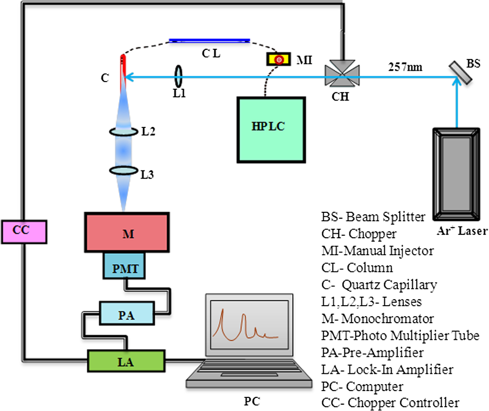 Saliva samples were diluted 20 to 50 times with prefiltered HPLC grade water. Hundred microliter freshly diluted samples were injected into the HPLC system with the 20 μl loop. Proteins were eluted under gradient run with A 70% to 50%, B 30% to 50% in 0 to 20 min, A 50% to 40%, B 50% to 60% in 25 min followed by B 60% to 100% in 26 to 30 min. After each sample run, the column was regenerated with water for 15 min. Prior to the injection of a sample, a blank run was recorded to ensure that the column was clean. 2.3.Data ProcessingData processing involves preprocessing of the data, principal component analysis (PCA), calculation of suitable parameters, and carrying out a match/no-match test of the parameters of test sample against parameters of standard calibration sets. The duration of each chromatogram is 30 min with the signal collection every 2 s; hence, each chromatogram has 900 data points. Preprocessing includes interpolation, smoothing, baseline correction, normalization, and alignment along the time axis. All data processing was done using PLSplus/IQ module of the GRAMS software (Thermo Scientific Inc., Rockford, IL). We have shown in our earlier studies on Raman and fluorescence spectra of tissues50–55 and protein profile studies of serum for ovarian, cervical, and breast malignancy conditions37,38 that the technique of match/no-match with statistical parameters of standard calibration sets from PCA is a very good method for discrimination between normal, premalignant, and malignant conditions. The method is described in detail in our earlier work. In brief, the method, like any other analytical method, uses standard calibration sets of each category, against which a test sample is matched using parameters derived from PCA. In the present work, standard calibration sets of protein profiles are formed using 10 to 15 saliva samples collected from subjects who have been judged to be normal/premalignant/malignant clinically and pathologically. They are subjected to PCA, and three parameters—scores of factors, squared sum of residuals (observed—simulated chromatogram)2, and M. distance34,36–39,52,53—are derived for the standard sets. Any test sample is then added to each calibration set, and the parameters of the test sample are compared with those of the calibration set. The sample is diagnosed as belonging to that set with which it matches within the range for that set for the decision-making threshold. 3.Results and DiscussionsFigure 2(a) shows typical preprocessed normal, malignant, and premalignant saliva chromatograms. Figure 2(b) contains all the three chromatograms expanded to five times showing several minor peaks. A closer look at these plots reveals that the noise level is such that a signal-to-noise ratio of 2 may correspond to a peak height of about 0.004 V. The peak around 1200 s is from -amylase. The signal for -amylase in this run is about 1 V. It was observed that in most of the chromatograms, this peak often goes out of the scale with the signal amplification. Higher values of amplification, PMT voltage, and laser power were used in all our runs to analyze and acquire information from smaller peaks in the chromatograms. Hence, the portion of the chromatogram belonging to -amylase was excluded for the PCA. It may be mentioned here, however, that the -amylase levels in saliva are also sensitive to disease conditions. The concentration of -amylase in saliva is about 19 to .56 This shows that our system has a detection limit of a few femtomoles of protein under present experimental conditions. This detection limit can be easily reduced by 1 to 2 orders of magnitude by appropriate use of laser power, for example multipassing and more efficient collection of fluorescence.57 Fig. 2(a) Typical preprocessed saliva chromatograms of normal, premalignant, and malignant classes (normalized with respect to 1200 s peak). (b) Expanded (five times) chromatograms in (a).  PCA was done with separate sections of the chromatograms, namely, in the regions of 400 to 650 s, 700 to 1100 s, 1400 to 1500 s, 1550– to 1750 s and also using complete chromatograms excluding -amylase peak. The choice of the regions were made on the basis of visual inspection by which it was found that these regions may contain the maximum information and give better results. It was observed that the third region above gives good sensitivity and specificity in comparison with the other regions/the complete chromatogram excluding -amylase peak. The significant number of factors was decided using the Eigen values, total percent variance, and squared residuals. Squared residual, as mentioned above, is the sum of squares of differences for all data points between observed and simulated chromatograms. The Mahalanobis distance (M. distance) is expressed in units of standard deviation.55 Receiver operating characteristic (ROC) curve analysis was done in an earlier study to find out the optimum value for M. distance58 for the classification of clinical samples. An M. distance of for a sample indicates the probability of the sample being in the same cluster with which the match was made to be , and a value gives a probability of a value . Hence, the samples with M. distance are classified as out of the calibration set. The PCA and match/no-match test results of region 3 are given in Tables 2Table 3–4 and the final results for other regions and complete chromatograms are shown in Table 5. Test runs were made using 10 factors. It was found that the first five factors contributed to about 98% of the total variance. It can be seen from Fig. 3 that first five factors’ contribution gives maximum variations, and from sixth factor onward the contribution can be attributed to random variations, which may include variations from day-to-day, noise, etc. The contributions from the higher factors are so small that they are not sensitive to sample changes. Table 2Prediction report using normal calibration test in the region 1400 to 1500 s.
Table 3Prediction report using malignant calibration test in the region 1400 to 1500 s.
Table 4Prediction report using premalignant calibration test in the region 1400 to 1500 s.
Table 5Results of all analyses.
In our method of PCA,52–54 the mean of data from all samples is first formed, and the variation of each sample from this mean is calculated. PCA is done with these variations. The variations from the mean for any sample are thus represented by its scores for the different factors. Thus, scores can be used in a first step as a discriminating parameter. Attempts were made to find the classification of samples by plotting the different scores along - and -axes and also by plotting scores of factors against the sample number. The plot of scores of factor 1 versus scores of factor 2 is shown in Fig. 4. From the figure, it can be seen that there is discrimination between normal and malignant samples; however, practically no decision can be made regarding premalignant samples simply based on the first two principal component scores. Much better discrimination can be achieved by using our match/no-match technique in which scores of factors, spectral residual, and M. distance are used as matching parameters. A standard calibration set of each class is formed using chromatograms from clinically/pathologically certified samples of that class. Parameters from these are used for the diagnosis of test samples for match/no-match test. If the parameters of a sample match with the parameters of the calibration set, the sample is considered to be of the same class as that of the test calibration set. If a sample does not belong to the class of the calibration set, the spectral residual and M. distance of the sample under test will be high compared with the ones that belong to the same class. Thus, by matching a given sample to each of the standard calibration sets, a more reliable classification can be achieved with good sensitivity and specificity. Table 2 shows the prediction report of the test made with the normal calibration set. It can be seen that almost all the normal samples lie in this range with the interference of only one malignant and a few premalignant samples representing a clear classification. ROC curve of two independent classes (premalignant and malignant) and the same for the combined diagnosis are shown in Fig. 5. Area under the curve calculated for premalignant, malignant, and combined () curve are 0.69, 0.89, and 0.74, respectively. From the plot, it is clear that using an M. distance value of 2 will give the best possible discrimination between the classes. Fig. 5Results of receiver operating characteristic (ROC) analysis with normal calibration set for the region 1400 to 1500 s. 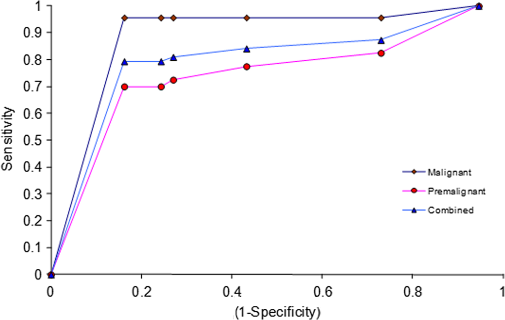 Table 2 shows that when tested with the normal calibration set, the majority of the normal samples match all malignant samples (except one), and a large number of premalignant samples do not match, giving much better discrimination between normal, premalignant, and malignant classes compared with the use of scores alone. All validation samples were subjected to the match/no-match test also with the malignant and premalignant standard sets. The results of tests made with malignant and premalignant calibration sets are shown in Tables 3 and 4, respectively. Table 5 lists the results of all the regions and the complete chromatograms for all the three classes. Only about 10 clinically/pathologically certified samples from each class were used to form the calibration sets. In the match/no-match test, every member of any standard calibration set is rotated out of the set and matched against the rest. Since the experimental system and mathematical data processing in the computer do not depend on the sample origin, the method is totally blind as to which sample (standard or validation) is involved. In other words, each member of the calibration set can also be considered as a validation sample. The sensitivity and specificity in the present studies, as seen from Table 5 are 79.37% and 77.38%, respectively. The positive and negative predictive values are 89.29% and 61.76%, respectively. Other methods like HPLC-mass spectrometry (MS), surface-enhanced laser desorption/ionization-MS, matrix-assisted laser desorption/ionization-MS, and sodium dodecyl sulfate-poly-acrylamide gel electrophoresis are available for protein profiling. These techniques have several limitations, discussed elsewhere.59,60 The reversed phase HPLC with ultra-sensitive LIF detection has been suggested as the best technique for diagnostic applications of protein profiling due to its superior resolution, high-time efficiency, high-detection capacity, and sensitivity.60 The combination of the highly sensitive LIF (which has advantages such as limited stray light effects, low background and accurate focusing capacity of the excitation source on to the micro-bore capillary leading to the excitation of picoliter amounts of samples without any loss of excitation energy etc.) and highly efficient HPLC enables easy detection of the ultra trace biomolecules in complex physiological samples. The other major advantage is the capability of detection of multiple markers in a single run with less time and a small quantity of the sample. Other groups have also studied salivary proteomes.61–63 Yamada et al.61 have studied salivary proteome, but no oral malignancy samples were investigated. No premalignant cases were investigated by Hu et al.62 Xie et al.63 have identified proteins in cells separated from saliva from four subjects with oral squamous cell carcinoma of tongue only and have not provided any diagnostic techniques. Almost all studies were done by mass spectroscopic techniques with the inherent disadvantages pointed out by Mohamed et al.60 The present study clearly shows that our technique of HPLC-LIF protein profiling-PCA pattern analysis of the profiles can provide a noninvasive, relatively fast, and sensitive method for screening for early detection. The same technique can, obviously, be used for monitoring the effectiveness of therapy and follow up for early detection of any regression after apparent cure. The method is extremely sensitive, and sensitivity can be increased further by 1 to 2 orders of magnitude,64 if necessary. 4.ConclusionFrom the present study, it can be concluded that protein profiling of saliva samples can be used as a screening technique for diagnosis of premalignant and malignant conditions of the oral cavity. As the method is noninvasive (no biopsy) and saliva can be easily obtained from the subject, the subject can be called back any number of times for cross-verification of any anomalies or abnormalities in the results. The technique is based on statistical analysis of instrumental data which can be completely automated and can be operated by a technician. It is thus highly adoptable for developing countries, where the majority of the population resides in areas with very limited hospital/clinical facilities. In the present study, we have used HPLC-LIF combined with PCA as a diagnostic tool for oral cancer screening. Out of the results from match/no-match test, it is observed that good discrimination can be achieved between normal/premalignant/malignant conditions. Using ROC analysis, it can be concluded that the M. distance with a value 2 will give the possible best discrimination of different classes. Though some suspicious premalignant cases may match normal/malignant conditions, any such cases can be called back for periodic examination at regular intervals (say, a few months) with only minimum efforts. Hence, the method can be used as a regular screening technique for the early detection of oral cancer. AcknowledgmentsAuthors are thankful to Manipal University for providing the research facility for the work. ReferencesA. Jemalet al.,
“Cancer statistics,”
CA Cancer J. Clin., 61
(2), 69
–90
(2011). http://dx.doi.org/10.3322/caac.v61:2 CAMCAM 0007-9235 Google Scholar
A. Jemalet al.,
“Global patterns of cancer incidence and mortality rates and trends,”
Cancer Epidemiol. Biomarkers Prev., 19 1893
–1907
(2010). http://dx.doi.org/10.1158/1055-9965.EPI-10-0437 CEBPE4 1055-9965 Google Scholar
R. W. Hinermanet al.,
“Post operative irradiation for squamous cell carcinoma of oral cavity: 35 year experience,”
Head Neck, 26
(11), 984
–994
(2004). http://dx.doi.org/10.1002/(ISSN)1097-0347 1043-3074 Google Scholar
S. KantolaM. ParikkaK. Jokinen,
“Prognostic factors in tongue cancer relative importance of demographic, clinical and histopathological factors,”
Br. J. Cancer, 83
(5), 614
–619
(2000). http://dx.doi.org/10.1054/bjoc.2000.1323 BJCAAI 0007-0920 Google Scholar
J. N. Myerset al.,
“Squamous cell carcinoma of tongue in adults: increasing incidence and factor that predict treatment outcomes,”
Otolaryng. Head Neck Surg., 122
(1), 44
–51
(2000). http://dx.doi.org/10.1016/S0194-5998(00)70142-2 OHNSDL 0194-5998 Google Scholar
N. Ramanujam,
“Fluorescence spectroscopy of neoplastic and non neoplastic tissues,”
Neoplasia, 2
(1–2), 89
–117
(2000). http://dx.doi.org/10.1038/sj.neo.7900077 1522-8002 Google Scholar
K. C. RibeiroL. P. KowalskiM. R. Latorre,
“Impact of comorbidity, symptoms and patients characteristics on prognosis of oral carcinomas,”
Otolaryng. Head Neck Surg., 126
(9), 1079
–1085
(2000). http://dx.doi.org/10.1001/archotol.126.9.1079 OHNSDL 0194-5998 Google Scholar
A. Sparanoet al.,
“Multivariate predictors of occult neck metastasis in early oral tongue cancer,”
Otolaryng. Head Neck Surg., 131
(4), 472
–476
(2004). http://dx.doi.org/10.1016/j.otohns.2004.04.008 OHNSDL 0194-5998 Google Scholar
C. CenterR. SiegelA. Jemal, Global Cancer Facts & Figures, 2nd ed.American Cancer Society, Atlanta
(2011). Google Scholar
I. AliW. A. WaniK. Saleem,
“Cancer scenario in India with future perspectives,”
Cancer Ther., 8 56
–70
(2011). CTCOE9 0896-5080 Google Scholar
S. K. Naiket al.,
“Optical screening of oral cancer: technology for emerging markets,”
2807
–2810
(2007). Google Scholar
B. W. Nevilleet al., Oral and Maxillofacial Pathology, 337
–369 2nd ed.WB Saunders, Philadelphia
(2002). Google Scholar
L. A. G. Rieset al., Cancer Statistics Review 1973–1988, National Cancer Institute, Bethesda, Maryland
(1991). Google Scholar
P. A. Swango,
“Cancers of the oral cavity and pharynx in the United States,”
J. Public Health Dent., 56
(6), 309
–318
(1996). http://dx.doi.org/10.1111/jphd.1996.56.issue-6 JPHDAC 0022-4006 Google Scholar
K. P. SchepmanI. Van der Waal,
“A proposal for classification and staging system for oral leukoplakia: a preliminary study,”
Oral Oncol., 31
(6), 396
–398
(1995). EJCCER 1368-8375 Google Scholar
J. E. BouquotB. S. Whitaker,
“Oral leukoplakia—rationale for diagnosis and prognosis of its clinical subtypes or ‘phases’,”
Quintessence Int., 25
(2), 133
–140
(1994). 0033-6572 Google Scholar
P. R. Murtiet al.,
“Malignant transformation rate in oral submucous fibrosis over a 17-year period,”
Community Dent. Oral Epidemiol., 13
(6), 340
–341
(1985). http://dx.doi.org/10.1111/com.1985.13.issue-6 CDOEAP 0301-5661 Google Scholar
P. C. Guptaet al.,
“Incidence rates of oral cancer and natural history of oral precancerous lesions in a 10 year follow up study of Indian villagers,”
Community Dent. Oral Epidemiol., 8
(6), 287
–333
(1980). http://dx.doi.org/10.1111/com.1980.8.issue-6 CDOEAP 0301-5661 Google Scholar
C. ScheifeleP. A. Reichart,
“Is there a natural limit of transformation rate of oral leukoplakia?,”
Oral Oncol., 39
(5), 470
–475
(2003). http://dx.doi.org/10.1016/S1368-8375(03)00006-X EJCCER 1368-8375 Google Scholar
M. N. Shiuet al.,
“Risk factors for leukoplakia and malignant transformation to oral carcinoma: a leukoplakia cohort in Taiwan,”
Br. J. Cancer, 82
(11), 1871
–1874
(2000). http://dx.doi.org/10.1054/bjoc.2000.1208 BJCAAI 0007-0920 Google Scholar
M. N. ShiuT. H. Chen,
“Intervention efficacy and malignant transformation to oral cancer among patients with leukoplakia,”
Oncol. Rep., 10
(6), 1683
–1692
(2003). OCRPEW 1021-335X Google Scholar
J. E. BouquotL. T. KurlandL. H. Wieland,
“Carcinoma in situ of the upper aerodigestive tract: incidence time trends and follow up in Rochester, Minnesota 1935-1984,”
Cancer, 61
(8), 1691
–1698
(1988). http://dx.doi.org/10.1002/(ISSN)1097-0142 CANCAR 1097-0142 Google Scholar
J. E. BouquotH. Ephros,
“Erythroplakia: the dangerous red mucosa,”
Pract. Periodontics Aesthet. Dent., 7
(6), 59
–68
(1995). Google Scholar
B. W. Nevilleet al., Oral and Maxillofacial Pathology, 3rd ed.Elsevier, St. Louis
(2009). Google Scholar
W. G. ShaferC. A. Waldron,
“Erythroplakia of the oral cavity,”
Cancer, 36
(3), 1021
–1028
(1975). http://dx.doi.org/10.1002/(ISSN)1097-0142 CANCAR 1097-0142 Google Scholar
P. M. SpeightP. R. Morgan,
“The natural history and pathology of oral cancer and pre cancer,”
Community Dent. Health, 10
(1), 31
–41
(1993). CDHEES Google Scholar
S. SilvermanM. GorskyF. Lozada,
“Oral leukoplakia and malignant transformation: a follow up study,”
Cancer, 53
(3), 563
–568
(1984). http://dx.doi.org/10.1002/(ISSN)1097-0142 CANCAR 1097-0142 Google Scholar
P. N. Sinolet al.,
“A case control study of oral submucous fibrosis with special reference to etiological role of areca nut,”
J. Oral Pathol. Med., 19
(2), 94
–98
(1990). http://dx.doi.org/10.1111/jop.1990.19.issue-2 JPMEEA 0904-2512 Google Scholar
R. Etzioniet al.,
“The case of early detection,”
Nat. Rev. Cancer, 3
(4), 243
–252
(2003). http://dx.doi.org/10.1038/nrc1041 NRCAC4 1474-175X Google Scholar
P. W. Smith,
“Fluorescence emission-based detection diagnosis of malignancy,”
J. Cell. Biochem., 87
(39), 54
–59
(2002). http://dx.doi.org/10.1002/(ISSN)1097-4644 JCEBD5 0730-2312 Google Scholar
K. Venkatakrishnaet al.,
“LIF-HPLC for detection of biomarkers in malignancy,”
in Proc. Natl. Laser Sym.,
323
(2000). Google Scholar
K. Venkatakrishnaet al.,
“Protein profiles in oral premalignancies: a laser spectroscopy study,”
in Proc. Natl. Laser Sym.,
345
(2001). Google Scholar
K. Venkatakrishnaet al.,
“HPLC-LIF for early detection of oral cancer,”
Curr. Sci., 84
(4), 551
–557
(2003). CUSCAM 0011-3891 Google Scholar
K. Venkatakrishnaet al.,
“Spit and polish for oral cancer test,”
News India (Nature),
(2003). Google Scholar
S. Menonet al.,
“Protein profile study of breast cancer using HPLC-LIF—a pilot study,”
Proc. SPIE, 6430 64300W
(2007). http://dx.doi.org/10.1117/12.699935 PSISDG 0277-786X Google Scholar
S. K. Singhet al.,
“Protein profile study of clinical samples of ovarian cancer using HPLC-LIF,”
Proc. SPIE, 6092 60920N
(2006). http://dx.doi.org/10.1117/12.647321 PSISDG 0277-786X Google Scholar
L. R. SujathaV. B. KarthaC. Santhosh,
“Protein profile study of serum of normal and cervical cancer subjects by high performance liquid chromatography-laser induced fluorescence,”
J. Biomed. Opt., 13
(5), 054062
(2008). http://dx.doi.org/10.1117/1.2992166 JBOPFO 1083-3668 Google Scholar
S. Bhatet al.,
“Protein profile analysis of cellular samples from the cervix for the objective diagnosis of cervical cancer using HPLC-LIF,”
J. Chromatogr. B, 878
(31), 3225
–3230
(2010). http://dx.doi.org/10.1016/j.jchromb.2010.09.025 1570-0232 Google Scholar
E. P. Diamandis,
“Proteomic patterns in biological fluids: do they represent the future of cancer diagnostics?,”
Clin. Chem., 49
(8), 1272
–1278
(2003). http://dx.doi.org/10.1373/49.8.1272 CLCHAU 0009-9147 Google Scholar
P. Dennyet al.,
“The proteomes of human parotid submandibular / sublingual gland salivas collected as the ductal secretions,”
J. Proteome Res., 7
(5), 1994
–2006
(2008). http://dx.doi.org/10.1021/pr700764j JPROBS 1535-3893 Google Scholar
C. F. Streckfuset al.,
“Breast cancer related proteins are present in saliva and are modulated secondary to ductal carcinoma in situ of the breast,”
Cancer Investig., 26
(2), 159
–167
(2008). http://dx.doi.org/10.1080/07357900701783883 CINVD7 0735-7907 Google Scholar
S. Huet al.,
“Salivary proteomics for oral cancer biomarker discovery,”
Clin. Cancer Res., 14 6246
–6252
(2008). http://dx.doi.org/10.1158/1078-0432.CCR-07-5037 CCREF4 1078-0432 Google Scholar
H. P. Lawrence,
“Salivary markers of systemic disease: non invasive diagnosis of disease and monitoring of general health,”
J. Can. Dent. Assoc., 68
(3), 170
–174
(2002). JCDAAS 0008-3372 Google Scholar
P. A. Wilmarthet al.,
“Two dimensional liquid chromatography study of human whole saliva proteome,”
J. Proteome Res., 3
(5), 1017
–1023
(2004). http://dx.doi.org/10.1021/pr049911o JPROBS 1535-3893 Google Scholar
D. T. Wong,
“Salivary diagnostics: enhancing disease detection and making medicine better,”
Eur. J. Dent. Educ., 12
(1), 22
–29
(2008). http://dx.doi.org/10.1111/eje.2008.12.issue-s1 1396-5883 Google Scholar
D. T. Wong,
“Towards a simple saliva-based test for the detection of the oral cancer,”
Expert Rev. Mol. Diagn., 6
(3), 267
–272
(2006). http://dx.doi.org/10.1586/14737159.6.3.267 1744-8352 Google Scholar
H. Xieet al.,
“Proteomics analysis of cells in whole saliva from oral cancer patients via value-added three-dimensional peptide fractionation and tandem mass spectrometry,”
Mol. Cell. Proteomics, 7
(3), 486
–498
(2007). http://dx.doi.org/10.1074/mcp.M700146-MCP200 MCPOBS 1535-9476 Google Scholar
B. Albertset al., Molecular Biology of the Cell, 1319 4th ed.Garland Publishing, Inc., New York
(2002). Google Scholar
R. J. Lakshmiet al.,
“Tissue Raman spectroscopy for the study of radiation damage: brain irradiation of mice,”
Radiat. Res., 157
(2), 175
–182
(2002). http://dx.doi.org/10.1667/0033-7587(2002)157[0175:TRSFTS]2.0.CO;2 RAREAE 0033-7587 Google Scholar
C. M. Krishnaet al.,
“Raman spectroscopy studies for diagnosis of cancers in human uterine cervix,”
Vib. Spectrosc., 41
(1), 136
–141
(2006). http://dx.doi.org/10.1016/j.vibspec.2006.01.011 VISPEK 0924-2031 Google Scholar
R. Maliniet al.,
“Discrimination of normal, inflammatory, premalignant, and malignant oral tissue: a Raman spectroscopy study,”
Biopolymers, 81
(3), 179
–193
(2006). http://dx.doi.org/10.1002/(ISSN)1097-0282 BIPMAA 0006-3525 Google Scholar
B. K. Manjunathet al.,
“Autofluorescence of oral tissue for optical pathology in oral malignancy,”
J. Photochem. Photobiol. B, 73
(1–2), 49
–58
(2004). http://dx.doi.org/10.1016/j.jphotobiol.2003.09.004 JPPBEG 1011-1344 Google Scholar
G. S. Nayaket al.,
“Principal component analysis and artificial neural network analysis of oral tissue fluorescence spectra: classification of normal premalignant and malignant pathological conditions,”
Biopolymers, 82
(2), 152
–166
(2006). http://dx.doi.org/10.1002/(ISSN)1097-0282 BIPMAA 0006-3525 Google Scholar
P. C. Mahalanobis,
“On the generalised distance in statistics,”
Proc. Natl. Inst. Sci. India, 2
(1), 49
–55
(1936). PNISBD 0370-0860 Google Scholar
D. S. Q. KohG. C. H. Koh,
“The use of salivary biomarkers in occupational and environmental medicine,”
Occup. Environ. Med., 64
(3), 202
–210
(2007). http://dx.doi.org/10.1136/oem.64.12.856-a OEMEEM 1351-0711 Google Scholar
S. Bhat,
“Protein profile and laser fluorescence spectroscopic studies of clinical samples for early detection of cervical cancer,”
Manipal University,
(2009). Google Scholar
A. Patilet al.,
“Evaluation of “high performance liquid chromatography -laser induced fluorescence (HPLC-LIF) for serum protein profiling for the early diagnosis of oral cancer,”
J. Biomed. Opt., 15
(6), 067007
(2010). http://dx.doi.org/10.1117/1.3523372 JBOPFO 1083-3668 Google Scholar
V. B. Karthaet al.,
“Diagnosis at the molecular level: analytical laser spectroscopy for clinical applications,”
in Photo/Electrochem. Photobiol.Environ. Energy Fuel,
153
–221
(2005). Google Scholar
G. S. Mohamedet al.,
“The importance of protein profiling in the diagnosis and treatment of hematologic malignancies,”
Turk. J. Hematol., 28 1
–14
(2011). http://dx.doi.org/10.5152/tjh. TJHSFS 1300-7777 Google Scholar
N. YamadaR. YujiE. Suzuki,
“The current status and future prospects of the salivary proteome,”
J. Health Sci., 55
(5), 682
–688
(2009). http://dx.doi.org/10.1248/jhs.55.682 JEHSDH 0360-1242 Google Scholar
S. Hu1et al.,
“Salivary proteomics for oral cancer biomarker discovery,”
Clin. Cancer Res., 14 6246
–6252
(2008). http://dx.doi.org/10.1158/1078-0432.CCR-07-5037 CCREF4 1078-0432 Google Scholar
H. Xieet al.,
“Proteomoics analysis of cells in whole saliva from oral cancer patients via value-added three-dimensional peptide fractionation and tandem mass spectrometry,”
Mol. Cell. Proteomics, 7 486
–498
(2007). http://dx.doi.org/10.1074/mcp.M700146-MCP200 MCPOBS 1535-9476 Google Scholar
A. Patilet al.,
“Highly sensitive high performance liquid chromatography-laser induced fluorescence for proteomics,”
ISRN Spectrosc., 2012 643979
(2012). http://dx.doi.org/10.5402/2012/643979 ISSPCD 2090-8776 Google Scholar
|