Analytical approaches for determining heat distributions and thermal criteria for infrared neural stimulation

Bryan J. Norton; Meghan A. Bowler; Jonathon D. Wells; Matthew D. Keller

doi:10.1117/1.JBO.18.9.098001

3 September 2013 Analytical approaches for determining heat distributions and thermal criteria for infrared neural stimulation

Bryan J. Norton, Meghan A. Bowler, Jonathon D. Wells, Matthew D. Keller

Author Affiliations +

Journal of Biomedical Optics, Vol. 18, Issue 9, 098001 (September 2013). https://doi.org/10.1117/1.JBO.18.9.098001

Abstract

Infrared neural stimulation (INS) is becoming an important complementary tool to electrical stimulation. Since the mechanism of INS is photothermal, describing the laser-induced heat distribution is fundamental to determining the relationship between stimulation pulses and neural responses. This work developed both a framework describing the time evolution of the heat distribution induced by optical fluence and a new method to extract thermal criteria (e.g., temperature change and rate of change) for neural activation. To solve the general problem of describing the temperature distribution, a Green’s function solution to the heat diffusion equation was determined and convolved with the optical fluence. This provided a solution in the form of a single integral over time, from which closed-form solutions can be determined for special cases. This work also yielded an expression for thermal relaxation time, which provides a rigorous description of thermal confinement for INS. The developed framework was then applied to experimental data from the cochlea to extract the minimum temperature increase and rate of that increase to stimulate the cochlear spiral ganglion. This result, and similar analyses applied to other neural systems, can then shed light on the fundamental mechanism for INS and aid the development of optical neuroprostheses.

1. Introduction

Infrared neural stimulation (INS) is a relatively new technique that is becoming an attractive complementary approach to conventional electrical nerve stimulation (ENS). It has now been demonstrated in numerous applications, including the cochlea,¹^–³ vestibular system,⁴ peripheral motor nerves,⁵^–⁷ facial nerve,⁸ vagus nerve,⁹ cavernous nerves of the prostate,¹⁰^,¹¹ somatosensory cortex,¹²^,¹³ and cardiomyocytes,¹⁴ among others. Depending on the application, INS offers several well-described advantages over ENS, including spatial precision, contact-free delivery, and lack of stimulation artifacts.¹⁵ However, two related limitations of INS, particularly for neural prosthesis use, are the low electrical-to-optical conversion efficiencies of infrared laser devices and the potentially damaging thermal effects of the stimulating beam.¹⁶ Since both of these limitations deal with heat deposition into tissue, minimizing optical (and thus electrical) energy usage while achieving neural stimulation is an important consideration.

The optimal INS parameters for several applications have been experimentally derived, but within the constraints of currently available laser sources. There is also little debate that the mechanism for INS is photothermal in nature,¹⁷^,¹⁸ but the exact underlying mechanism remains unclear. Several studies have demonstrated contributions to the action of INS by membrane capacitance changes,¹⁹ transient receptor potential (TRP) channels,²⁰ and intracellular calcium ion transients,²¹ though the relative importance of each of these in various cell types has not yet been elucidated. Regardless of the cellular mechanism, no clear understanding of the minimum thermal criteria, such as temperature change and rate of temperature change at the excitable tissue, for safe and effective INS exists at this time.

Due to the difficulty of performing precise, parametric studies to investigate the thermal aspects of INS in vivo, there has been recent interest in applying numerical simulations to provide insight. In a work by Thompson et al.²²^,²³ and previous work by the authors,²⁴ Monte Carlo simulations were used to determine photon distributions in tissue for typical INS experiments, and finite element analysis was then performed to determine heat distributions. This kind of analysis can be very useful for investigating peak temperatures and general temperature distributions in tissue as needed to examine general device safety, but it does not provide significant insight into how these temperature changes lead to neural activation.

The goal of this work was thus to develop an analytical approach to thermal changes during INS that can predict what thermal changes (e.g., temperature increase and rate of increase) are necessary for neural activation. The approach does not depend on the specific cellular mechanism of INS, but its identified thermal parameters for a given application can help evaluate the validity of proposed mechanisms.¹⁹^–²¹ The approach is broken into three sections. In the first (Sec. 2 of the manuscript), a three-dimensional expression for the time evolution of the temperature profile resulting from the absorption of an optical beam is presented. This is a general analytic solution, unlike thermal models that rely on finite element analysis. Most importantly, it delivers a set of equations used in the subsequent section to invert the stimulation problem to find thermal criteria for stimulation.

A simple set of assumptions compatible with current knowledge of INS is then proposed in Sec. 3, and thermal variables within this model are investigated. Specifically, we are interested in how stimulation depends on pulse width, energy, peak power, and stimulation geometry. Finally, the framework to extract thermal stimulation criteria is applied to cochlear INS data from Richter et al. at Northwestern University in Sec. 4. Although additional work to validate this analysis with in vivo work is required, in general, this kind of analysis should inform future decisions on INS device parameters such as spot size, pulse width, pulse energy, stimulation frequency, and stimulation depth. More efficient, and therefore feasible, devices will be realized.

2. General Solution

2.1.

Theoretical Framework

In this section, the problem of determining the temperature distribution that results from absorption of light in a medium is considered. In the case that absorption dominates scattering, the radial fluence distribution in the medium follows the incident radiant exposure distribution. The depth dependence takes the form of a decaying exponential. This is the case for INS because wavelengths have been chosen to have strong absorption in tissue, such that the intense localization of temperature produces stimulation.⁷^,¹⁷ Single-mode optical beams propagating in free space have a strictly Gaussian intensity distribution. Optical beams from highly multimode sources (e.g., multimode optical fibers) are not strictly Gaussian but, as a result of greater propagation attenuation for high mode angle light, tend toward a Gaussian-shaped envelope. An acceptable and desirably simple representation of the fluence in tissue is thus a radially Gaussian distribution with decaying exponential depth intensity. To determine the temperature distribution, the heat diffusion equation is needed.

Eq. (1)

\frac{\partial T}{\partial t} = α^{2} (\frac{\partial^{2} T}{\partial x^{2}} + \frac{\partial^{2} T}{\partial y^{2}} + \frac{\partial^{2} T}{\partial z^{2}}) + f (t) \frac{γ P}{4 π^{2} a b} e^{\frac{- x^{2}}{2 a^{2}}} e^{\frac{- y^{2}}{2 b^{2}}} e^{- γ z},

where

T

is the temperature,

t

is time,

α

is diffusivity,

x

and

y

are spatial coordinates transverse to light propagation,

z

is the spatial coordinate longitudinal to light propagation,

γ

is the attenuation coefficient (

z

coordinate),

P

is instantaneous power,

a

is the radius of heat distribution (

x

coordinate), and

b

is the radius of heat distribution (

y

coordinate).

In the above partial differential equation, the diffusion rate (left hand side) is driven by the sum of the curvature of the distribution and the heat load (right hand side). No algebraic or transcendental expression describes the solution to this equation. Instead, a Green’s function formalism can provide insight.

Taking the heat diffusion equation for a point heat source in Cartesian $R^{3}$ and time leads to

Eq. (2)

\frac{\partial g}{\partial t} = α^{2} (\frac{\partial^{2} g}{\partial x^{2}} + \frac{\partial^{2} g}{\partial y^{2}} + \frac{\partial^{2} g}{\partial z^{2}}) + δ (x - x^{'}) δ (y - y^{'}) δ (z - z^{'}) δ (t - t^{'}) .

Finding a solution to the above partial differential equation provides a description of the temperature distribution resulting from a point source of heat. This description can be used to find specific solutions to any general heat distribution. The full derivation is left to the Appendix, but the solution takes the form of

Eq. (3)

g (x, y, z, t | x^{'}, y^{'}, z^{'}, t^{'}) = \frac{1}{{[4 π α^{2} (t - t^{'})]}^{\frac{2}{3}}} e^{- [\frac{{(x - x^{'})}^{2}}{4 α^{2} (t - t^{'})} + \frac{{(y - y^{'})}^{2}}{4 α^{2} (t - t^{'})} + \frac{{(z - z^{'})}^{2}}{4 α^{2} (t - t^{'})}]} .

This solution describes the time evolution of a unit impulse of heat. Note that the spatial distribution is Gaussian in shape. The specific source distribution can be treated by convolving the Green’s function with the distribution of interest (in this case, the inhomogeneous term of the partial differential equation).

Eq. (4)

T (x, y, z, t) = \frac{γ P}{2 π a b ρ C} \int_{0}^{t} \int_{0}^{\infty} \int_{- \infty}^{\infty} \int_{- \infty}^{\infty} \frac{f (t^{'})}{{[4 π α^{2} (t - t^{'})]}^{\frac{2}{3}}} e^{\frac{- {x^{'}}^{2}}{2 a^{2}}} e^{\frac{- {y^{'}}^{2}}{2 b^{2}}} e^{- γ z^{'}} e^{- [\frac{{(x - x^{'})}^{2}}{4 α^{2} (t - t^{'})} + \frac{{(y - y^{'})}^{2}}{4 α^{2} (t - t^{'})} + \frac{{(z - z^{'})}^{2}}{4 α^{2} (t - t^{'})}]} d x^{'} d y^{'} d z^{'} d t^{'},

where

ρ

is the density of tissue, and

C

is the specific heat of tissue.

The three spatial convolutions have closed-form solutions that yield an integral solution for temperature at any point in space and time, given by

Eq. (5)

T (x, y, z, t) = \frac{P γ e^{- γ z}}{4 π ρ C b^{2}} \int_{0}^{t} f (t^{'}) \frac{e^{\frac{- (x^{2} + y^{2})}{2 b^{2} + 4 α^{2} (t - t^{'})} + γ^{2} α^{2} (t - t^{'})}}{1 + {(\frac{α}{b})}^{2} (t - t^{'})} erfc [\frac{2 γ α^{2} (t - t^{'}) + z}{\sqrt{4 α^{2} (t - t^{'})}}] d t^{'},

Within the suppressed derivation, $a$ has been set equal to $b$ , forcing the optical spot to be round in profile. This has been done to make the resulting expression simpler, but was not necessary to perform the convolutions. The result is an integral expression for the temperature resulting from a Gaussian-shaped heat distribution anywhere in space or time for any arbitrary optical pulse format. It is worth noting that this is an exact solution to the heat diffusion equation for the assumed heat distribution, with no additional limiting assumptions or approximation, resulting in an expression that is useful in all applications with similar heat distributions. As discussed below, powerful insight can be gained from some useful approximations that yield analytic expressions.

2.2.

Special Cases

For some interesting idealized cases, fully analytic solutions exist. These solutions are at the heart of the benefit of this approach, and significant insight can be gained by understanding the following expressions.

2.2.1.

Fast pulse

The assumption that the laser pulse is much shorter in duration than the rate of diffusion can be expressed by representing the time dependence of the fluence as a delta function $f (t^{'}) = δ (t^{'})$ . This yields

Eq. (6)

T {(x, y, x, t)}_{F ast} = \frac{P γ e^{- γ z}}{4 π ρ C b^{2}} \frac{e^{\frac{- (x^{2} + y^{2})}{2 b^{2} + 4 α^{2} t} + γ^{2} α^{2} t}}{1 + t {(\frac{α}{b})}^{2}} erfc [\frac{2 γ α^{2} (t) + z}{\sqrt{4 α^{2} (t)}}] .

2.2.2.

Thermal confinement limit

Thermal confinement occurs when heat is being deposited into a system in a time interval much shorter than that during which significant diffusion occurs. This can be expressed by taking the limit as $t \to t^{'}$ .

Eq. (7)

T {(x, y, x, t)}_{Conf} = \lim_{t \to t'} \frac{P γ e^{- γ z}}{4 π ρ C b^{2}} \int_{0}^{t} f (t^{'}) \frac{e^{\frac{- (x^{2} + y^{2})}{2 b^{2} + 4 α^{2} (t - t')} + γ^{2} α^{2} (t - t^{'})}}{1 + {(\frac{α}{b})}^{2} (t - t^{'})} erfc [\frac{2 γ α^{2} (t - t^{'}) + z}{\sqrt{4 α^{2} (t - t^{'})}}] d t^{'},

Eq. (8)

T {(x, y, z, t)}_{Conf} = \frac{P γ e^{- γ z}}{4 π ρ C b^{2}} e^{\frac{- (x^{2} + y^{2})}{2 b^{2}}} \int_{0}^{t} f (t^{'}) d t^{'} .

2.3.

Thermal Time Constant

The thermal time constant is a useful concept for characterizing a thermal system. The thermal time constant is the amount of time the system takes to relax to $1 / e$ its initial state $T (t = 0) / e = T (t = τ_{1 / e})$ . This relaxation time depends not only on the thermal properties of the medium, but also on the specific distribution of the heat load. As a result, its accurate representation requires nothing less than the preceding analysis. By combining Eq. (6) with the definition of the thermal time constant above, the following equality is produced:

Eq. (9)

\frac{1}{e} = \frac{e^{γ^{2} α^{2} τ_{1 / e}} erfc (γ α \sqrt{τ_{1 / e}})}{1 + {(\frac{α}{b})}^{2} τ_{1 / e}},

where

τ_{1 / e}

is the thermal time constant.

This expression can be solved for time numerically to determine the thermal time constant. Figure 1 is a graphical representation of finding the thermal time constant of brain tissue, whose properties are summarized in Table 1. From this solution, it takes the system 67 ms to decay to its $1 / e$ value, and the deposited heat is 95% contained for up to 764 μs. This result is a strong justification that the optically induced heat distribution is thermally confined for experimental pulse durations $< 700 μ s$ .

Fig. 1

Log plot of thermal relaxation in brain tissue [Eq. (6)]. Horizontal lines mark the points at which the temperature has decayed to 95% ( $τ_{95 %}$ ) and $1 / e$ [ $τ_{1 / e}$ ; see Eq. (9)] of the initial maximum value, which was arbitrarily set to 1°C.

Table 1

Parameters of brain tissue and heat distribution.

	Quantity	Symbol	Value
Brain tissue:	Density	$ρ$	$1040 kg / m^{2}$
	Specific heat	$C$	$3650 J / Kg ° C$
	Thermal conductivity	$k$	$0.527 W / m ° C$
	Diffusivity	$α^{2} = k / ρ C$	$1.3 \times 10^{- 7} m^{2} / s$
Heat distribution:	Attenuation coefficient	$γ$	$35.2 {cm}^{- 1}$
	Distribution radius	$b$	0.01 cm

2.4.

Idealized Response in INS Applications

Figure 2 profiles the thermal response of a laser pulse in the regime in which the heat is essentially completely confined to the irradiation zone during the pulse, as defined from Fig. 1. During the pulse, diffusion is negligible, so the temperature increases linearly to a maximum value determined by the pulse energy and with a slope determined by peak power. After enough time has passed for diffusion to be significant, the temperature rolls off in accordance with the fast pulse approximation. These analyses can be applied to any application in which heat is delivered to a homogeneous material fast enough to be thermally confined, which includes all known current INS applications.

Fig. 2

Pictorial representation of idealized thermal response over time to a fast optical pulse that deposits all of its energy into the tissue as heat before any thermal relaxation may occur.

Specifically for cochlear INS, reports from Richter and colleagues indicate that the most relevant pulse widths for future optical cochlear implant development are in the range of $\sim 20$ to 200 μs,²⁵^–²⁷ which satisfy both the thermal confinement and fast pulse criteria discussed above. Although longer pulse durations (and therefore lower peak powers) can be used successfully, they require a greater amount of total energy deposition to produce neural responses of equivalent magnitude.²⁵^–²⁷ To minimize the effects of tissue heating and prolong potential battery life, the shorter pulse durations become more relevant; thus, the remainder of the manuscript focuses on the $20$ to 200 μs range of pulse durations.

3. Thermal Variable Investigation

3.1.

Assumptions and Definitions

Using the established framework, the relationship between stimulation pulse parameters and activated neural tissue can be investigated, beginning with simplifying assumptions about a chosen population of neurons. Assumptions of the neural activation model include the following:

1. Two thermal criteria must be met for neural activation: a sufficient increase in temperature at the excitable tissue caused by the optical pulse, $Δ T_{c}$ , and an appropriately quick rate of that temperature increase, ${\dot{T}}_{c}$ (C/s). If only one or neither of these criteria is met, the cell will not fire.
2. The two aforementioned thermal criteria are independent.
3. The cell population is spatially homogenous.
4. The relationship between compound action potential (CAP) and number of activated neurons is linear.
Eq. (10)
$CAP \propto Γ \int d V ρ_{g} (x, y, z) H (x, y, z, T > T_{c}) * H (x, y, z, \frac{\partial T}{\partial t} > {\dot{T}}_{c}),$
where $Γ$ is the voltage scaling factor, $V$ is the volume, $ρ_{g}$ is the neuron density, $T_{c}$ is the temperature criterion, and ${\dot{T}}_{c}$ is the temperature rate criterion. The thermal criteria are encoded as Heaviside functions.
Eq. (11)
$H (x, y, z, T > T_{c}) = 1; H (x, y, z, T < T_{c}) = 0; H (x, y, z, \frac{\partial T}{\partial t} > {\dot{T}}_{c}) = 1; H (x, y, z, \frac{\partial T}{\partial t} < {\dot{T}}_{c}) = 0 .$

The objective is to determine thermal criteria necessary for neural stimulation. Simplifying the dynamics sufficiently to isolate one criterion at a time is accomplished by designing experiments to eliminate as many complicating variables as possible. For the case of the current neural activation model, addressing one criterion at a time makes the problem of extracting values tenable. To this end, the problem is broken up into two cases: one corresponding to the temperature increase criterion and one for the rate of temperature increase criterion. Case 1 assumes the temperature rate criterion is satisfied, which corresponds to an instantaneous pulse of finite energy (infinite peak power). Case 2 assumes the temperature increase criterion is satisfied, which corresponds to a pulse of infinite energy with finite peak power. These idealizations are not fully achievable experimentally, but to induce the desired behavior, one only needs to dramatically oversatisfy the criteria.

3.2.

Case 1: Temperature Rate Criterion Satisfied

Assuming the temperature rate criterion, ${\dot{T}}_{c}$ , is satisfied,

Eq. (12)

H (x, y, z, \frac{\partial T}{\partial t} > {\dot{T}}_{c}) = 1 .

The resulting CAP integral is then

Eq. (13)

CAP \propto ρ_{g} \int H (x, y, z, T > T_{c}) d V .

Converting the Green’s function solution to cylindrical coordinates and setting the temperature to an arbitrary criterion,

T_{c}

, the stimulation boundaries are defined by

Eq. (14)

T_{c} = \frac{P_{Peak} γ t}{4 π ρ C b^{2}} e^{\frac{- r^{2}}{2 b^{2}}} e^{- γ z},

where

P_{Peak}

is the peak optical power.

One can then solve for the depth of stimulation, $z_{c}$ , and the radius of stimulation, $r_{c}$ , as follows:

Eq. (15)

z_{c} = \frac{1}{γ} [\ln (\frac{P_{Peak} γ t}{4 π T_{c} ρ C b^{2}}) - \frac{r^{2}}{2 b^{2}}],

Eq. (16)

r_{c} = b \sqrt{2 \ln (\frac{P_{Peak} γ t}{4 π ρ C T_{c} b^{2}}) - 2 γ z_{0}} .

As depicted in Fig. 3, the volume of interest is a paraboloid truncated by the distance to the neural tissue boundary, $z_{0}$ . The CAP response is described by the following integral, where the criteria for stimulation (i.e., $z_{c}$ and $r_{c}$ ) are carried in the integrand and limits, respectively, thus negating the need to integrate over $d z$ as well.

Eq. (17)

CAP = Γ ρ_{g} \int_{0}^{2 π} \int_{0}^{r_{c}} (z_{c} - z_{0}) r d r d ϕ,

Eq. (18)

CAP = Γ ρ_{g} \frac{π b^{2}}{λ} {[\ln (\frac{P_{Peak} t γ}{4 π T_{c} ρ C b^{2}}) - z_{o} γ]}^{2} .

Fig. 3

Graphical representation of optical source and stimulation volume paraboloid. The neural tissue lies a distance $z_{0}$ axially from the optical fiber, and the stimulated paraboloid has initial radius $b$ and subsequent radius 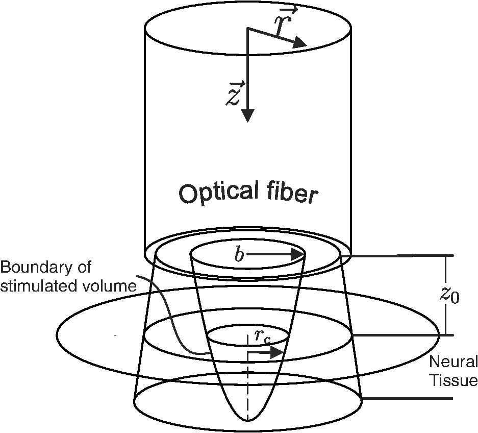$r_{c}$ .

The above CAP growth function includes a geometrically driven threshold where no CAP exists if the temperature criteria are not satisfied deeper than $z_{o}$ . Assuming a continuous distribution of cells allows contributions by arbitrarily small volumes of cells just deeper than $z_{o}$ to be included in the CAP. For large stimulated volumes, this idealization may be acceptable, but for low pulse energy, it is inaccurate. The probabilistic nature of the neurons being activated and the experimental noise floor (i.e., one cannot detect neural activity below a certain level) are neglected here as well. All of this leads to an additional threshold behavior not taken into account within this model. An additional threshold was therefore included from the outset as a method to represent relevant behavior not consistent with the continuous model.

Eq. (19)

CAP = Γ ρ_{g} \frac{π b^{2}}{γ} {\ln [\frac{(E_{Pulse} - E_{0}) γ}{4 π T_{c} ρ C b^{2}}] - z_{o} γ}^{2} .

By shifting the energy domain over by $E_{0}$ , we are merely encoding the fact that for some low energy values (below $E_{0}$ ), no CAP will be observed.

To illustrate the geometry expressed by the above analysis, Fig. 3 depicts the optical source and resulting parabolic volume of stimulated tissue. As discussed previously, within thermal confinement, the optical distribution and heat load have the same geometry. The approximate boundary of the optical distribution is represented in Fig. 3 as rays passing through the tissue. The radius of the fluence distribution is represented as $b$ . The distance between the optical source and the neural tissue is $z_{o}$ . Volume within the stimulation boundary, but shallower than $z_{o}$ , does not contribute to the CAP. The radius of stimulation at the boundary of the neural tissue is represented by $r_{Stim}$ .

3.3.

Case 2: Temperature Criterion Satisfied

Assuming the temperature criterion, $Δ T_{c}$ , is satisfied,

Eq. (20)

H (x, y, z, T > T_{c}) = 1 .

The resulting CAP integral becomes

Eq. (21)

CAP \propto ρ_{g} \int H (x, y, z, \frac{\partial T}{\partial t} > {\dot{T}}_{c}) d V .

The temperature criteria expression differs only in that it is the derivative of the one used in case 1 [Eq. (14)].

Eq. (22)

{\dot{T}}_{c} = \frac{P_{Peak} γ}{4 π ρ C b^{2}} e^{\frac{- r^{2}}{2 b^{2}}} e^{- γ z} .

For the rest of this case, the arguments are identical to case 1. The results of each case are summarized in Table 2.

Table 2

Summarized thermal relations for the two stimulation cases.

	Case 1	Case2
Description:	Instantaneous pulse with finite energy	Infinite energy with finite peak power
Assumed criteria:	$H [(\partial T / \partial t) > {\dot{T}}_{c}]$	$H (T > T_{c})$
CAP relation:	$CAP \propto \int H [(\partial T / \partial t) > {\overset{}{T}}_{c}] d V$	$CAP \propto \int H (T > T_{c}) d V$
Thermal criteria:	${\dot{T}}_{c} = P_{Peak} γ / 4 π ρ C b^{2} e^{- γ^{2} / 2 b^{2}} e^{- γ z}$	$T_{C} = E_{Pulse} γ / 4 π ρ C b^{2} e^{- γ^{2} / 2 b^{2}} e^{- γ z}$
CAP growth function:	$CAP \propto Γ ρ_{g} {\ln {[(P_{Peak} - P_{0}) γ / 4 π T_{c} ρ C b^{2}] - z γ}}^{2}$	$CAP \propto Γ ρ_{g} (π b^{2} / γ) {\ln [(E_{Pulse} - E_{0}) γ / 4 π T_{c} ρ C b^{2}] - z γ}^{2}$

In case 1 ( $Δ T_{c}$ limited), the CAP response is limited by pulse energy. Thus, in the case where heat is imparted to the neural tissue sufficiently fast to satisfy the rate criteria, the response is only dependent on pulse energy. In case 2 ( ${\dot{T}}_{c}$ limited), the CAP response is limited by peak power. It follows that in the case where the temperature of the tissue is raised above the temperature criteria, the CAP response is limited by peak power. This case is far more difficult to manifest experimentally. In case 1, the rate criteria can be satisfied for the entire stimulation volume because the pulse can be delivered instantaneously. In case 2, there is a time period during which the tissue temperature is increasing, but the criterion ( $Δ T_{c}$ ) is not satisfied; this results from the fact that the required tissue temperature cannot be reached instantaneously.

Figure 4 depicts a set of radial temperature (solid line) and temperature rate (dotted line) distributions for different relative stimulation sizes. The distinguishing values are the radius of stimulation limited by the temperature criteria, $r_{T_{c}}$ , and the radius of stimulation limited by the temperature rate criteria, $r_{{\dot{T}}_{c}}$ . The first case ( $r_{T_{c}} > r_{{\dot{T}}_{c}}$ ) represents the instance in which the stimulation is limited by peak power. In this case, the tissue that meets the temperature criterion, but is outside $r_{{\dot{T}}_{c}}$ , is wasted heat, which is represented by the shaded regions of the distribution. The second case ( $r_{T_{c}} < r_{{\dot{T}}_{c}}$ ) represents the instance in which the stimulation is limited by pulse energy. This case does not waste any energy in the stimulation but uses more peak power than is strictly necessary. This is likely to have a detrimental impact on the optical stimulation system. The third case ( $r_{T_{c}} = r_{{\dot{T}}_{c}}$ ) wastes neither energy nor peak power because the criteria shells are the same physical size. It also leads to an interesting and useful relationship.

Eq. (23)

r_{T_{c}} = r_{{\dot{T}}_{c}} \Rightarrow P_{Peak} = E_{Pulse} (\frac{{\dot{T}}_{c}}{T_{c}}),

where

E_{Pulse}

is the optical pulse energy.

Fig. 4

Graphical representation of peak power and pulse energy stimulation widths. Top panel shows the case where the radius of the region in which the temperature criterion is satisfied ( $r_{T_{c}}$ ) is larger than the region in which the rate change criterion ( $r_{{\dot{T}}_{c}}$ ) is satisfied. Middle panel shows the opposite of the top, in which the rate change criterion is satisfied over a larger region than the temperature criterion. Bottom panel shows the optimal case where the criteria are equally met.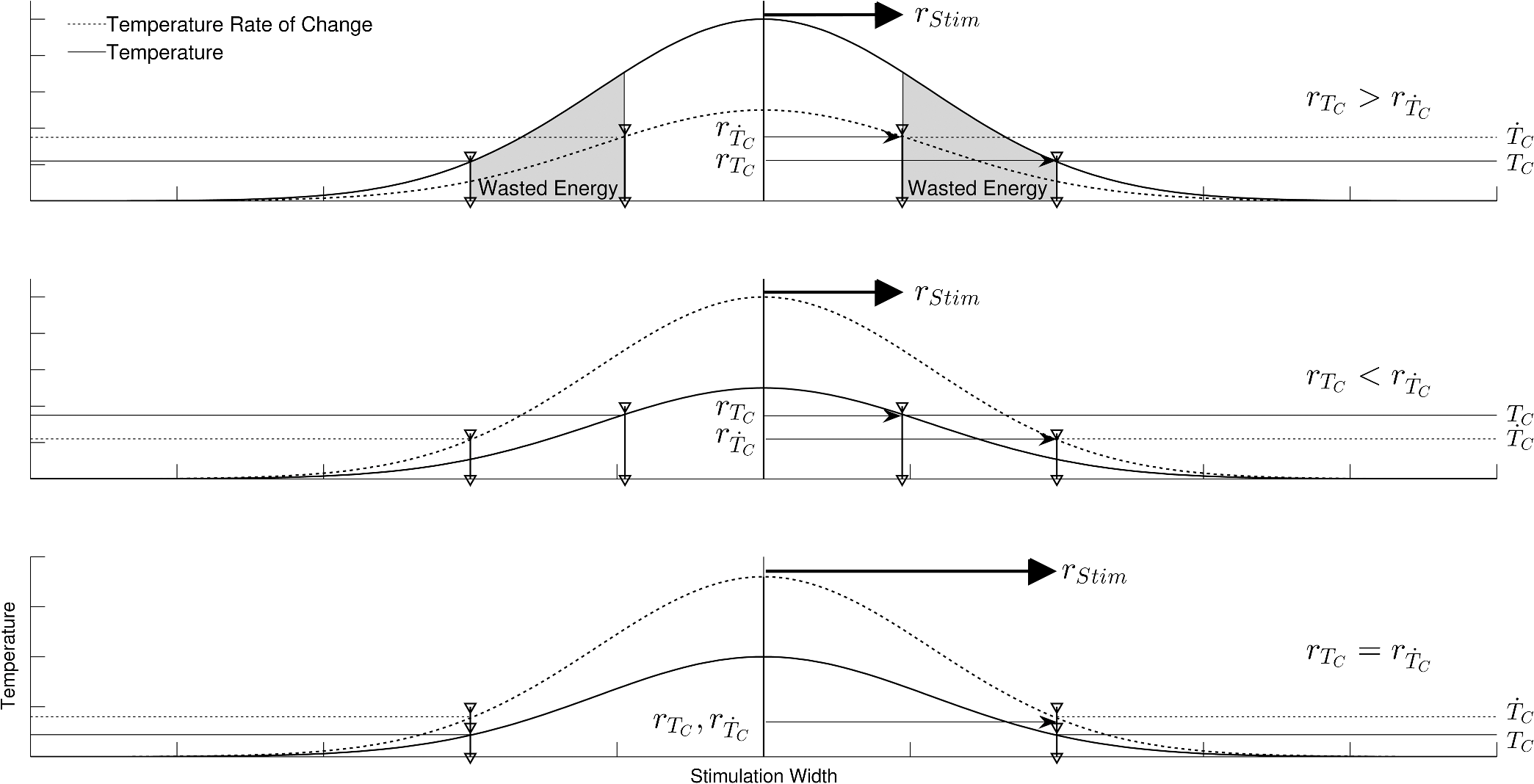

This formula relates the two thermal criteria, providing a way to determine the rate given the activation temperature. The parameter values for which the two shells are equal can be found experimentally. By collecting data at a constant pulse energy (constant temperature profile) and increasing the peak power, the CAP response will flatten when the limited shells cross. The transition point will be the equal volume parameter set. Just as important is the ability to determine the pulse width associated with efficient use of energy and peak power (i.e., none wasted). This ideal time is simply the ratio of the critical temperature to the temperature rate.

Eq. (24)

τ_{pulse width} = (\frac{T_{c}}{{\dot{T}}_{c}}),

where

τ_{pulse width}

is the optical pulse width where simulation is limited by temperature and temperature rate.

4. Extraction of Key Cochlear Stimulation Parameters

As a test case, this section uses in vivo data from INS of spiral ganglion cells in the cat cochlea provided by Richter et al. at Northwestern University. As shown in Fig. 5, these data consist of CAP amplitudes as a function of pulse energy for a series of pulse durations ranging from 20 to 200 μs. The data were gathered similarly to how the same group produced Fig. 3 from Richter et al.,²⁶ Fig. 5 from Izzo et al.,²⁷ and Fig. 3 from Rajguru et al.²⁵ The one difference is that the previous figures used radiant exposure ( ${J / cm}^{2}$ ) on the $x$ axis, whereas Fig. 5 simply uses pulse energy since all measurements used the same spot size. Comparing this experimental data with the model cases then enables the determination of whether INS, at least in the cochlea, is pulse energy or peak power limited.

Fig. 5

In vivo data from Richter et al. demonstrating the growth of CAP responses in cats as a function of pulse energy for a series of pulse durations.

4.1.

Extracting $T_{c}$

In vivo electrophysiology data can be plagued with noise and inconsistencies as a result of the experimental difficulty resulting from live animal testing. Thus, the conclusions drawn here will be restricted to broad behavior. The amplitude of the CAP response in Fig. 5 saturates as the pulse width is decreased below 60 μs. This result is dependent on case 1 being satisfied (pulse energy limited). To test this conclusion as suggested above, the data are replotted in both energy and peak power domains in Fig. 6.

Fig. 6

Comparison of experimental CAP responses from selected data in Fig. 5 in (a) peak power and (b) pulse energy domains.

It is clear from Fig. 6 that INS with the depicted range of pulse widths is significantly more pulse energy limited than peak power limited. The pulse energy representation results in a significantly smaller standard deviation than the peak power representation ( $σ_{E} < σ_{P}$ ). The average of the 20, 40, 50, and 60 μs data was then used to extract the temperature criterion, $T_{c}$ . A parameter search was performed to minimize the difference between the CAP growth function and the pulse energy–limited experimental data, as seen in Fig. 7. This provides the values for $a_{1}$ through $a_{3}$ (note that $a_{4}$ in Fig. 7 represents the $z γ$ product from the CAP expression in Table 2 and is thus not an extracted value), which are shown in Table 3. There is particular interest in $a_{3}$ because it gives the value of $T_{c}$ , which comes out to $\sim 0.8 mK$ as the minimum temperature change criterion.

Fig. 7

Comparison of experimental data from Fig. 6(b) and CAP growth model using extracted thermal criteria (values in Table 3). The red dashed line represents the pulse energy below which no neural activity can be detected, even if it is elicited.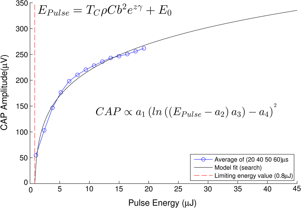

Table 3

Table of extracted values from Fig. 7.

	Relationship	Value extracted	Symbol	Criteria values
$a_{1}$	$a_{1} = Γ π ρ_{g} b^{2} / γ$	5 μV	$Γ ρ_{g}$	$159.1 kg / {As}^{3}$
$a_{2}$	$a_{2} = E_{0}$	0.83 μV	$E_{0}$	0.83 μJ
$a_{3}$	$a_{3} = γ / T_{c} ρ C b^{2}$	$115.12 {μ J}^{- 1}$	$T_{c}$	0.8 mK

Although this value seems quite low, it represents a minimum for one criterion to be met, and in practice, most of the irradiated tissue volume reaches higher temperatures. This low minimum temperature criterion also suggests that the more practical limiting criterion for neural activation in the cochlea (which is known to have significantly lower radiant exposure thresholds for INS than other tissues) would be the rate of temperature increase, ${\dot{T}}_{c}$ , as discussed in Sec. 4.2. To put the 0.8 mK value in perspective, though, Fig. 8 displays calculated isothermal lines for a series of pulse energies from a 200 μm diameter fiber with tissue properties from Table 1. The maximum temperature rises induced even right by the fiber tip (lower left corner of plots) are very small, given the low pulse energies, and by the time photons pass through a typical amount of tissue between the fiber and neural cells, the temperature increases at the neural tissue are even smaller. By examining the area under the 0.8 mK curve that falls within the neural tissue volume, one can see the expected trend consistent with Fig. 7.

Fig. 8

Temperature distribution in tissue immediately following 1, 5, and 10 μJ optical pulses from a 200 μm diameter fiber placed at the lower left of the plots. All properties are the same as from Table 1. The 500 μm distance between the fiber tip and neural tissue represents a typical amount of non-neural tissue that must be penetrated.

4.2.

Extracting ${\dot{T}}_{c}$

As described above, experimentally satisfying the requirements for case 2 is not trivial, if at all possible. However, the peak power saturation point (Fig. 9) can be used to determine the ratio of the two criteria. As depicted in Fig. 9, holding pulse energy constant within thermal confinement and increasing peak power results in a consistent temperature shell throughout the experiment. As the peak power shell increases in size and eventually eclipses the pulse energy shell, the limiting criterion switches from power to energy. At this transition point, the two shells are the same size, and the peak power and pulse energy are related by the ratio of the two criteria. Experimentally, these data are available from the CAP versus energy plot (Fig. 5). In Fig. 10, slices of the data have been taken for constant energy and increasing peak power. This plot expresses the desired behavior: each of the pulse energy plots saturates at a unique value. The transition point for each pulse energy value and other relevant values are summarized in Table 4.

Fig. 9

Conceptual representation of CAP saturation behavior dependence on peak power at constant energy. The marked point represents the transition point between pulse energy– and peak power–limited responses.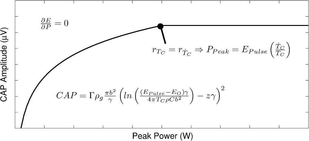

Fig. 10

Representation of experimental data in the peak power domain with constant pulse energy. Heavy markers note the peak power at which the CAP growth saturates for each noted series of pulse energy.

Table 4

Saturation points for each pulse energy.

$E_{Pulse}$ (μJ)	$P_{Peak}$ (W)	$τ_{width} = T_{c} / {\dot{T}}_{c}$ (μs)
10	0.2	50
15	0.3	50
20	0.4	50
25	0.5	50
30	0.5	63

Extracting ${\dot{T}}_{c}$ is then a simple matter of finding the temperature rate criterion from the temperature criterion (Table 5). Thus, the optimal pulse width ( $\sim 50 μ s$ ), temperature increase criterion ( $> 0.8 mK$ ), and the temperature rate criterion ( $\sim 15 K / s$ ) for INS in the cochlea have all been determined.

Table 5

Extracted thermal criteria.

$〈 T_{c} / {\dot{T}}_{c} 〉$ (μs)	$T_{c}$ (mK)	${\dot{T}}_{c}$ (K/s)
53	0.8	15.1

4.3.

Spot Size

Understanding the relationships that control stimulation allows the optimization of optical spot size. This is of interest because it affects not only the safety and perceived loudness of a potential optical cochlear implant, but also the required beam shaping and stimulator system power. The radius of the stimulation heat load, $b$ , plays two roles in the CAP growth function [Eq. (18)]: first, as a term inside the natural log and second, as a multiplicative amplitude factor. The spot size’s role inside the log is related to the minimum input required for stimulation. The multiplicative amplitude dependence of spot size tells us about how the stimulation cross-section relates to nerve cell recruitment growth.

4.3.1.

Minimum criteria for stimulation

The $1 / e$ stimulation radius’s ( $b$ ) role inside the log describes the minimum penetration depth to stimulate neurons. The assumption for this is that the natural log term is larger than the depth term. The inequality below [Eq. (25)] must be satisfied for the stimulation shell to reach the neural tissue. Here, the specific energy or power variables, as well as the temperature or rate criteria, are replaced with a placeholder ( $O p$ and ${Therm}_{c}$ , respectively) to represent both concepts. This prevents redundant statements.

Eq. (25)

\ln [\frac{(O p_{input} - O p_{0}) γ}{(4 π ρ C b^{2}) {Therm}_{C}}] - z_{0} γ > 0,

where

O p_{input}

is the general optical input and

{Therm}_{C}

is the general thermal criteria.

This relation then sets requirements on $b$ (the $1 / e$ heat load radius).

Eq. (26)

0 < b^{2} < \frac{(O p_{input} - O p_{0}) γ}{(4 π ρ C) {Therm}_{C}} e^{- z_{o} γ} .

Per unit of optical input, as the distance from the source to the neural tissue, $z$ , increases, the radius of stimulation must decrease in order to have the photon concentration necessary to reach the neural tissue. In contrast, as the optical input increases, the acceptable radius also increases. This can be considered an energy or power density criterion with one addendum: it is not with respect to raw input, but that which is above the threshold introduced in Sec. 2.

Eq. (27)

\frac{O p_{input} - O p_{0}}{A_{1 / e}} > \frac{(4 ρ C) {Therm}_{C}}{γ} e^{z_{o} γ} .

Here, $A_{1 / e}$ is the area defined by $b$ , the $1 / e$ radius of the heat distribution ( $A_{1 / e} = π b^{2}$ ).

4.3.2.

Recruitment growth

The overall amplitude factor of $b^{2}$ reflects the fact that recruitment gained by increasing the radius of stimulation requires less energy than doing so by increasing the depth (i.e., depth recruitment costs more than width). The most efficient stimulation comes from the largest spot possible that satisfies the power and energy density equation [Eq. (27)]. The limit to this is the width of the neural population; if the thermal profile is above threshold [see Eq. (16)] outside this region, that heat is being wasted. Similarly, if the thermal profile is above threshold [see Eq. (15)] deeper than the neural cells exist, heat is again wasted.

Figure 11 depicts a family of iso-CAP curves plotted in terms of required optical input and spot size to maintain a constant CAP. The family is framed by the stimulation threshold limit on the bottom, the depth of the neural population for small spot sizes, and the width of the neural population limit for larger spots. In general, larger spot sizes require less optical input for equal CAP. The point at which the range switches from being limited by depth to width is where the maximum dynamic range achievable without wasting optical energy is found. However, this may not represent the optimal spot size in every application. For some applications, a somewhat smaller dynamic range may be acceptable and achievable by using a larger spot with significantly less optical input.

Fig. 11

Family of iso-CAP curves depicting the relationship between optical input (i.e., power or energy) and spot size to maintain the same neural response. These are overlaid with limits imposed by the stimulation threshold, the depth of the neural population, and the width of the neural population. The maximum dynamic range occurs at the intersection of the depth and width limits.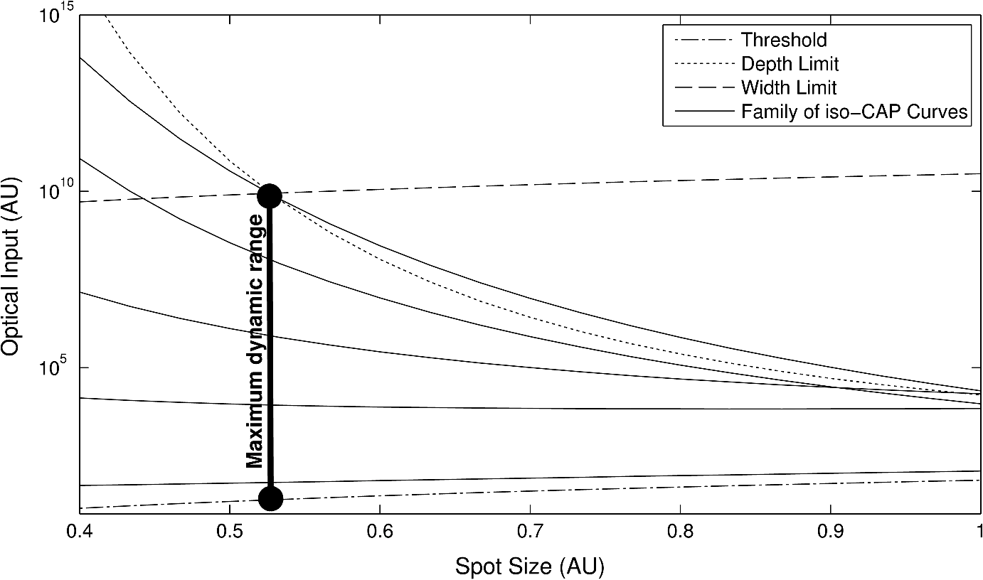

5. Discussion

This work has provided an analytical framework for a deeper understanding of the thermal criteria required for infrared neural stimulation. In particular, it has shown that in the cochlea, INS requires a laser pulse that provides a minimal but rapid temperature increase. This finding supports many previous studies focused on understanding the mechanism of INS. Wells et al. first demonstrated that a change in temperature, rather than an absolute temperature, was a key factor for initiating INS. The authors measured temperature profiles with peripheral nerves at normal body and lowered temperatures and saw no differences in neural responses for identical increases from the different baseline temperatures.¹⁷ Rajguru et al. saw similar results in the vestibular system of toadfish at normal and lowered body temperatures.⁴

The Northwestern group has published several pieces of data supporting the specific cochlear result. In Moreno et al., they note that no temperature change could be detected in a thermochromic ink prep (sensitivity of $\sim 1 ° C$ ) with typical INS pulse energies,²⁸ and in Izzo et al., they calculate that the maximum temperature rise from a typical stimulation pulse at the spiral ganglion cells should be $< 0.1 ° C$ .²⁷ As noted in Sec. 2.4, several reports from Northwestern have also shown that for a fixed pulse energy, longer pulse durations that provide slower heating evoke smaller neural responses than shorter pulse durations.²⁵^–²⁷

The dependence on the rate of temperature change also largely aligns with the work of Shapiro et al. in examining membrane capacitance changes during INS.¹⁹ Using artificial bilayers, HEK cells, and Xenopus oocytes, they showed that the rapid temperature change induced by infrared pulses alters the ionic double layers around the plasma membranes, thus altering the total membrane capacitance and causing a depolarization.¹⁹ The magnitude of the capacitance change is fairly small though ( $\sim 8 %$ max), and the authors noted that cells expressing the requisite sodium and potassium channels to fire an action potential had to be brought close to threshold for infrared pulses to evoke an action potential.¹⁹ To investigate this finding further, Peterson and Tyler modeled the magnitudes of capacitance changes required for cells to be stimulated via this mechanism.²⁹ They found that regardless of beam diameter, pulse width, and dependence on illuminating nodes of Ranvier, it was unlikely that the capacitance change alone would be responsible for INS, though they hypothesize that it does play some important role.²⁹ It is also possible that the effect of capacitance changes is different in different cell types due to variations in physiology, such as presence and thickness of myelin.

In contrast to the above studies, others have suggested that absolute temperature changes are required for neural activation from infrared stimulation. For example, Fried et al. have been able to observe functional responses from both pulsed and continuous wave irradiation of the rat cavernous nerves of the prostate, provided that the nerve is heated to the same temperature of $\sim 43 ° C$ .³⁰^,³¹ This temperature is in the range where one would expect the TRPV family of cation channels to be relevant, particularly TRPV1, which is typically given an activation temperature of 43°C.³² Indeed, Albert et al. demonstrated that TRPV4 was vital to INS of cultured retinal and vestibular ganglion cells,²⁰ and Bec et al. followed up with a study showing that for different wavelengths and pulse durations, the stimulation thresholds depended largely on absolute temperature achieved. It should be noted that the activation temperature of TRPV4 is $\sim 27 ° C$ ,³² though, so one could reasonably expect a different role for TRPV4 during in vitro studies with baseline temperatures $< 27 ° C$ (such as Albert et al.,²⁰ Bec et al.,¹⁸ and portions of Liljemalm et al.³³) and in vivo studies with warmer baseline temperatures, where TRPV4 may be constitutively active.³² The in vitro studies¹⁸^,²⁰^,³³ have also shown consistently higher radiant exposure thresholds, and therefore peak temperatures, compared with in vivo stimulation. The reasons for this discrepancy are currently unclear.

The other primary focus for the cellular mechanism of INS stems from work by Dittami et al., who showed that intracellular calcium ions, likely released from the mitochondria, were the key element for INS in cardiomyocytes.²¹ They demonstrated this result by selectively blocking various calcium transporters in the mitochondrial membrane, some of which are also known to block TRP channels. Previous studies in cardiomyocytes also demonstrated the ability to thermally stimulate them via mitochondrial release of calcium in the absence of any extracellular calcium,³⁴ which further supports the lack of TRP channel involvement.

Given the various findings to date, it is difficult to speculate on whether there exists a single cellular mechanism by which infrared light stimulates excitable tissue, or whether different cell types respond via different mechanisms. It seems likely that some findings (i.e., membrane capacitance, TRP channels, intracellular calcium) could be reconciled in at least some cell types with further physiological studies. The analytical framework presented here may be useful in evaluating such mechanisms as well. By applying the same approach taken in Sec. 4 to similarly gathered data from other cell types, one could understand how important absolute temperature changes are versus the rate of those changes for the particular application. Knowing the exact cellular mechanism is not necessary to use this framework to benefit device design and development though. Given proper experimental data, one can easily extract $T_{c}$ and ${\dot{T}}_{c}$ , which enables the determination of the optimal pulse width such that the stimulation zone is equally limited by peak power and pulse energy, thus achieving the most efficient stimulation.

Future work should focus on verifying these preliminary results in vivo. Thermal criteria should be investigated at even lower pulse widths to confirm that at least the lower range of pulse widths follows the pulse energy–limited trend in the cochlea. Other neural populations should be investigated as well to determine any differences in their thermal criteria and behavior. Future models may use a more nuanced heat distribution to more closely approximate the effects of scattering. In addition, temperature criteria such as these can be used in conjunction with Monte Carlo scattering models and finite element analyses to provide the area of stimulation in more complicated, biologically relevant geometries. These formalisms and methods would then allow the construction of much more efficient INS devices.

Appendices

Appendix

A detailed solution of the problem described and solved in Sec. 2 is provided. The goal was to solve the heat diffusion equation driven by a Gaussian heat distribution in $x$ and $y$ , and exponentially attenuated by $γ$ in $z$ below.

Eq. (28)

\frac{\partial T}{\partial t} - α^{2} (\frac{\partial^{2} T}{\partial x^{2}} + \frac{\partial^{2} T}{\partial y^{2}} + \frac{\partial^{2} T}{\partial z^{2}}) = f (t^{'}) \frac{γ P_{Peak}}{4 π^{2} a b} e^{\frac{- {x^{'}}^{2}}{2 a^{2}}} e^{\frac{- {y^{'}}^{2}}{2 b^{2}}} e^{- γ z^{'}} .

The difference between the rate of relaxation and the curvature of the temperature distribution is the heat load; the driving force is the curvature. We first solve for a point heat source in Cartesian $R^{3}$ and time. The heat diffusion equation is

Eq. (29)

\frac{\partial g}{\partial t} - α^{2} (\frac{\partial^{2} g}{\partial x^{2}} + \frac{\partial^{2} g}{\partial y^{2}} + \frac{\partial^{2} g}{\partial z^{2}}) = α^{2} δ (x - x^{'}) δ (y - y^{'}) δ (z - z^{'}) δ (t - t^{'}) .

We perform a Laplace transform in time because we are interested in time after the initial heat load delivery and we perform a Fourier transform in $x$ and $y$ because we are interested in all space along the $x$ and $y$ axes. This yields an ordinary differential equation (ODE) in $z$ .

Eq. (30)

\frac{d^{2} \bar{G}}{d z^{2}} - (k^{2} - \frac{s}{α^{2}}) \bar{G} = δ (z - z^{'}) e^{- i k x^{'} - i l y^{'} - s t^{'}} .

We solve this ODE in two parts, the homogenous solution (when $z \neq z^{'}$ ) and the discontinuity (when $z = z^{'}$ ).

Eq. (31)

\frac{d^{2} \bar{G}}{d z^{2}} - (κ^{2} - \frac{s}{α^{2}}) \bar{G} = 0 .

The general solution to this equation is

Eq. (32)

\bar{G} = A_{1} e^{- γ z + β} + A_{2} e^{γ z + β},

where

Eq. (33)

γ = \sqrt{k^{2} + \frac{s}{α^{2}}} .

To solve the inhomogeneous equation, we integrate over the discontinuity at $z = z^{'}$ .

Eq. (34)

\int_{z^{'} - ε}^{z^{'} + ε} \frac{d^{2} \bar{G}}{d z^{2}} d z - (k^{2} - \frac{s}{a^{2}}) \int_{z^{'} - ε}^{z^{'} + ε} \bar{G} d z = e^{- i k x^{'} - i l y^{'} - s t^{'}} \int_{z^{'} - ε}^{z^{'} + ε} δ (z - z^{'}) d z .

First, $G$ must be piecewise smooth. This is true because a temperature distribution cannot be discontinuous. This implies

Eq. (35)

\lim_{ε \to 0} \int_{z' - ε}^{z' + ε} \bar{G} d z = 0 if {\bar{G}}_{z' - ε} = {\bar{G}}_{z' + ε} .

Second, we know by definition that

Eq. (36)

\lim_{ε \to 0} \int_{z^{'} - ε}^{z^{'} + ε} δ (z - z^{'}) d z = 1 .

Third, the slope of the distribution at the discontinuity is defined by the following:

Eq. (37)

\int_{z^{'} - ε}^{z^{'} + ε} \frac{d^{2} \bar{G}}{d z^{2}} d z = \frac{d \bar{G}}{d z} |_{z^{'} - ε}^{z^{'} + ε} .

Given these relationships, the inhomogeneous ODE reduces to

Eq. (38)

\frac{d \bar{G}}{d z} |_{z^{'} - ε}^{z^{'} + ε} = {\bar{G^{'}}}_{z^{'} + ε} - {\bar{G^{'}}}_{z^{'} - ε} = e^{- i k x^{'} - i l y^{'} - s t^{'}} .

Assuming $G^{'}$ on each side of $z^{'}$ is a linearly independent solution to the homogeneous equation,

Eq. (39)

{\bar{G^{'}}}_{z^{'} - ε} = A_{1} γ e^{(z - z^{'}) γ + β} and {\bar{G^{'}}}_{z^{'} + ε} = - A_{2} γ e^{- (z - z^{'}) γ + β} .

Eq. (40)

As ε \to 0, {\frac{d \bar{G}}{d z} |}_{z^{'} - ε}^{z^{'} + ε} = A_{1} γ e^{(z^{'} + ε - z^{'}) γ + β} + A_{2} γ e^{- (z^{'} - ε - z^{'}) γ + β}

reduces to

Eq. (41)

{\frac{d \bar{G}}{d z} |}_{z^{'} - ε}^{z^{'} + ε} = A_{1} γ e^{β} + A_{2} γ e^{β} .

By combining Eqs. (38) and (41), we know that

Eq. (42)

A_{1} γ e^{β} + A_{2} γ e^{β} = e^{- i k x^{'} - i γ y^{'} - s t^{'}} .

By inspection, we find

Eq. (43)

β = - i k x^{'} - i γ y^{'} - s t^{'} and A_{1} γ + A_{2} γ = 1 .

We know $A_{1} = A_{2}$ because yielding $A_{1} = 1 / 2 γ$ . Now that we know how each side of the discontinuity is shaped, we can combine the solutions to obtain a single function defining the transformed solution.

Eq. (44)

\bar{G} = \frac{e^{- | z - z^{'} | \sqrt{k^{2} + \frac{s}{α^{2}}} - i k x^{'} - i l y^{'} - s t^{'}}}{2 \sqrt{k^{2} + \frac{s}{α^{2}}}} .

Now that we have a complete transformed solution for Eq. (30), we must transform it back to the space and time domain. Taking the inverse Laplace and Fourier transforms of the solution to the ODE will give us the Green’s function for the diffusion equation.

Eq. (45)

g (x, y, z, t | x^{'}, y^{'}, z^{'}, t^{'}) = \frac{1}{{[4 π α^{2} (t - t^{'})]}^{\frac{2}{3}}} e^{- (\frac{{(x - x^{'})}^{2}}{4 α^{2} (t - t^{'})} + \frac{{(y - y^{'})}^{2}}{4 α^{2} (t - t^{'})} + \frac{{(z - z^{'})}^{2}}{4 α^{2} (t - t^{'})})} .

The optical pulse is a finite heat source, so we can treat it as a distribution of point heat sources. We can merge the distribution of heat sources with the diffusion of a single point source in a convolution integral.

Eq. (46)

T (x, y, z, t) = \frac{1}{ρ C} \int_{0}^{t} \int_{0}^{\infty} \int_{- \infty}^{\infty} \int_{- \infty}^{\infty} f (x^{'}, y^{'}, z^{'}, t^{'}) g (x, y, z, t | x^{'}, y^{'}, z^{'}, t^{'}) d x^{'} d y^{'} d z^{'} d t^{'} .

We represent the heat distribution as a function Gaussian in $x$ and $y$ and exponentially attenuated by $γ$ in $z$ .

Eq. (47)

f (x^{'}, y^{'}, z^{'}, t^{'}) = f (t^{'}) \frac{γ P_{Peak}}{2 π a b} e^{\frac{- {x^{'}}^{2}}{2 a^{2}}} e^{\frac{- {y^{'}}^{2}}{2 b^{2}}} e^{- γ z^{'}} .

Our convolution integral is thus

Eq. (48)

T (x, y, z, t) = \frac{γ P_{Peak}}{2 π a b ρ C} \int_{0}^{t} \int_{0}^{\infty} \int_{- \infty}^{\infty} \int_{- \infty}^{\infty} \frac{f (t^{'})}{{[4 π α^{2} (t - t^{'})]}^{\frac{2}{3}}} e^{\frac{- {x^{'}}^{2}}{2 a^{2}}} e^{\frac{- {y^{'}}^{2}}{2 b^{2}}} e^{- γ z^{'}} e^{- [\frac{{(x - x^{'})}^{2}}{4 α^{2} (t - t^{'})} + \frac{{(y - y^{'})}^{2}}{4 α^{2} (t - t^{'})} + \frac{{(z - z^{'})}^{2}}{4 α^{2} (t - t^{'})}]} d x^{'} d y^{'} d z^{'} d t^{'} .

According to Gradshteyn and Ryzhik, we have the following spatial convolutions:

Eq. (49)

f (x^{'}) \otimes g (x^{'}) = \int_{- \infty}^{\infty} e^{\frac{- {x^{'}}^{2}}{2 a^{2}}} e^{\frac{- {(x - x^{'})}^{2}}{4 α^{2} (t - t^{'})}} d x^{'} = \frac{\sqrt{π}}{\sqrt{\frac{1}{4 a^{2} (t - t^{'})} - \frac{1}{2 a^{2}}}} e^{\frac{α x^{2}}{1 - 4 α a^{2} (t - t^{'})}} f (y^{'}) \otimes g (y^{'}) = \int_{- \infty}^{\infty} e^{\frac{- {y^{'}}^{2}}{2 a^{2}}} e^{\frac{- {(y - y^{'})}^{2}}{4 α^{2} (t - t^{'})}} d x^{'} = \frac{\sqrt{π}}{\sqrt{\frac{1}{4 a^{2} (t - t^{'})} - \frac{1}{2 b^{2}}}} e^{\frac{α y^{2}}{1 - 4 α a^{2} (t - t^{'})}} f (z^{'}) \otimes g (z^{'}) = \int_{0}^{\infty} e^{- γ z^{'}} e^{\frac{- {(z - z^{'})}^{2}}{4 α^{2} (t - t^{'})}} d z^{'} = \frac{\sqrt{4 π α^{2} (t - t^{'})}}{2} e^{γ^{2} α^{2} (t - t^{'}) + γ z} erfc [\frac{2 γ α^{2} (t - t^{'}) - z^{'}}{\sqrt{4 α^{2} (t - t^{'})}}] .

These convolutions yield an analytical solution for temperature at any point, given a time of inspection, $t$ , and the timing of pulses, $f (t^{'})$ .

Eq. (50)

T (x, y, z, t) = \frac{P_{Peak} γ e^{- γ z}}{4 π ρ C b^{2}} \int_{0}^{t} f (t^{'}) \frac{e^{\frac{- (x^{2} + y^{2})}{2 b^{2} + 4 α^{2} (t - t^{'})} + γ^{2} α^{2} (t - t^{'})}}{1 + {(\frac{α}{b})}^{2} (t - t^{'})} erfc [\frac{2 γ α^{2} (t - t^{'}) + z}{\sqrt{4 α^{2} (t - t^{'})}}] d t^{'} .

Assuming a single instantaneous pulse at $t = 0$ , we have $f (t') = δ (t')$ . Evaluation of the convolution with this idealization yields

Eq. (51)

T (x, y, x, t) = \frac{P_{Peak} γ e^{- γ z}}{4 π ρ C b^{2}} \frac{e^{\frac{- (x^{2} + y^{2})}{2 b^{2} + 4 α^{2} t} + γ^{2} α^{2} t}}{1 + t {(\frac{α}{b})}^{2}} erfc [\frac{2 γ α^{2} (t) + z}{\sqrt{4 α^{2} (t)}}] .

To find the thermal confinement limit, we examine the time immediately after the pulse, or when $(t - t^{'}) = 0$ . Thermal confinement means taking the limit such that ( $t - t'$ ) is small.

Eq. (52)

T {(x, y, x, t)}_{Conf} = \lim_{t \to t^{'}} \frac{P_{Peak} γ e^{- γ z}}{4 π ρ C b^{2}} \int_{0}^{t} f (t^{'}) \frac{e^{\frac{- (x^{2} + y^{2})}{2 b^{2} + 4 α^{2} (t - t^{'})} + γ^{2} α^{2} (t - t^{'})}}{1 + {(\frac{α}{b})}^{2} (t - t^{'})} erfc [\frac{2 γ α^{2} (t - t^{'}) + z}{\sqrt{4 α^{2} (t - t^{'})}}] d t^{'} .

Eq. (53)

T {(x, y, z, t)}_{Conf} = \frac{P_{Peak} γ e^{- γ z}}{4 π ρ C b^{2}} e^{\frac{- (x^{2} + y^{2})}{2 b^{2}}} \int_{0}^{t} f (t) d t^{'} .

We evaluate this at $(x, y, z) = (0, 0, 0)$ since the peak temperature will exist at the center of the distribution at the depth closest to the heat source.

Eq. (54)

T {(t)}_{Conf} = \frac{P_{Peak} γ}{4 π ρ C b^{2}} \int_{0}^{t} f (t) d t .

Acknowledgments

We would like to thank Lockheed Martin Corporate Engineering and Technology and Lockheed Martin MS2 for financial support of this work. We would also like to thank Dr. Claus-Peter Richter for providing the in vivo data from his cochlear INS experiments.

References

1.

A. I. Maticet al., “Behavioral and electrophysiological responses evoked by chronic infrared neural stimulation of the cochlea,” PLoS ONE, 8 (3), e58189 (2013). http://dx.doi.org/10.1371/journal.pone.0058189 1932-6203 Google Scholar

2.

C. P. Richteret al., “Spread of cochlear excitation during stimulation with pulsed infrared radiation: inferior colliculus measurements,” J. Neural Eng., 8 (5), 056006 (2011). http://dx.doi.org/10.1088/1741-2560/8/5/056006 1741-2560 Google Scholar

3.

A. D. Izzoet al., “Laser stimulation of the auditory nerve,” Laser Surg. Med., 38 (8), 745 –753 (2006). http://dx.doi.org/10.1002/(ISSN)1096-9101 LSMEDI 0196-8092 Google Scholar

4.

S. M. Rajguruet al., “Infrared photostimulation of the crista ampullaris,” J. Physiol., 589 (6), 1283 –1294 (2011). http://dx.doi.org/10.1113/tjp.2011.589.issue-6 JPHYA7 0022-3751 Google Scholar

5.

J. Wellset al., “Pulsed laser versus electrical energy for peripheral nerve stimulation,” J. Neurosci. Methods, 163 (2), 326 –337 (2007). http://dx.doi.org/10.1016/j.jneumeth.2007.03.016 JNMEDT 0165-0270 Google Scholar

6.

J. D. Wellset al., “Optical stimulation of neural tissue in vivo,” Opt. Lett., 30 (5), 504 –506 (2005). http://dx.doi.org/10.1364/OL.30.000504 OPLEDP 0146-9592 Google Scholar

7.

J. D. Wellset al., “Application of infrared light for in vivo neural stimulation,” J. Biomed. Opt., 10 (6), 064003 (2005). http://dx.doi.org/10.1117/1.2121772 JBOPFO 1083-3668 Google Scholar

8.

I. U. Teudtet al., “Optical stimulation of the facial nerve: a new monitoring technique?,” Laryngoscope, 117 (9), 1641 –1647 (2007). http://dx.doi.org/10.1097/MLG.0b013e318074ec00 LARYA8 0023-852X Google Scholar

9.

A. Y. Rheeet al., “Photostimulation of sensory neurons of the rat vagus nerve,” Proc. SPIE, 6854 68540E (2008). http://dx.doi.org/10.1117/12.772037 PSISDG 0277-786X Google Scholar

10.

N. M. Friedet al., “Laser stimulation of the cavernous nerves in the rat prostate, in vivo: optimization of wavelength, pulse energy, and pulse repetition rate,” in Conf. Proc. IEEE Engineering in Medicine and Biology Society, 2777 –2780 (2008). Google Scholar

11.

N. M. Friedet al., “Noncontact stimulation of the cavernous nerves in the rat prostate using a tunable-wavelength thulium fiber laser,” J. Endourol., 22 (3), 409 –413 (2008). http://dx.doi.org/10.1089/end.2008.9996 JENDE3 0892-7790 Google Scholar

12.

J. M. Cayceet al., “Pulsed infrared light alters neural activity in rat somatosensory cortex in vivo,” Neuroimage, 57 (1), 155 –166 (2011). http://dx.doi.org/10.1016/j.neuroimage.2011.03.084 NEIMEF 1053-8119 Google Scholar

13.

J. M. Cayceet al., “Functional characterization of infrared neural stimulation in non-human primate cortex,” in Photonic Therapeutics and Diagnostics VIII, Photonics West, (2012). Google Scholar

14.

M. W. Jenkinset al., “Optical pacing of the embryonic heart,” Nat. Photon., 4 (9), 623 –626 (2010). http://dx.doi.org/10.1038/nphoton.2010.166 1749-4885 Google Scholar

15.

C. P. Richteret al., “Neural stimulation with optical radiation,” Laser Photon. Rev., 5 68 –80 (2010). http://dx.doi.org/10.1002/lpor.200900044 Google Scholar

16.

J. D. Wellset al., “Optically mediated nerve stimulation: identification of injury thresholds,” Lasers Surg. Med., 39 (6), 513 –526 (2007). http://dx.doi.org/10.1002/(ISSN)1096-9101 LSMEDI 0196-8092 Google Scholar

17.

J. D. Wellset al., “Biophysical mechanisms of transient optical stimulation of peripheral nerve,” Biophys. J., 93 (7), 2567 –2580 (2007). http://dx.doi.org/10.1529/biophysj.107.104786 BIOJAU 0006-3495 Google Scholar

18.

J. M. Becet al., “Characteristics of laser stimulation by near infrared pulses of retinal and vestibular primary neurons,” Lasers Surg. Med., 44 (9), 736 –745 (2012). http://dx.doi.org/10.1002/lsm.v44.9 LSMEDI 0196-8092 Google Scholar

19.

M. G. Shapiroet al., “Infrared light excites cells by changing their electrical capacitance,” Nat. Commun., 3 736 (2012). http://dx.doi.org/10.1038/ncomms1742 NCAOBW 2041-1723 Google Scholar

20.

E. S. Albertet al., “TRPV4 channels mediate the infrared laser-evoked response in sensory neurons,” J. Neurophysiol., 107 (12), 3227 –3234 (2012). http://dx.doi.org/10.1152/jn.00424.2011 JONEA4 0022-3077 Google Scholar

21.

G. M. Dittamiet al., “Intracellular calcium transients evoked by pulsed infrared radiation in neonatal cardiomyocytes,” J. Physiol., 589 (6), 1295 –1306 (2011). http://dx.doi.org/10.1113/tjp.2011.589.issue-6 JPHYA7 0022-3751 Google Scholar

22.

A. C. Thompsonet al., “Modeling of the temporal effects of heating during infrared neural stimulation,” J. Biomed. Opt., 18 (3), 035004 (2013). http://dx.doi.org/10.1117/1.JBO.18.3.035004 JBOPFO 1083-3668 Google Scholar

23.

A. C. Thompsonet al., “Modeling of light absorption in tissue during infrared neural stimulation,” J Biomed Opt., 17 (7), 075002 (2012). http://dx.doi.org/10.1117/1.JBO.17.7.075002 JBOPFO 1083-3668 Google Scholar

24.

M. D. Kelleret al., “Multi-physics system performance model for numerical simulations of infrared nerve stimulation,” in Photons and Neurons III, Photonics West, (2011). Google Scholar

25.

S. M. Rajguruet al., “Optical cochlear implants: evaluation of surgical approach and laser parameters in cats,” Hear Res., 269 (1–2), 102 –111 (2010). http://dx.doi.org/10.1016/j.heares.2010.06.021 HERED3 0378-5955 Google Scholar

26.

C.-P. Richteret al., “Optical stimulation of auditory neurons: effects of acute and chronic deafening,” Hear Res., 242 (1–2), 42 –51 (2008). http://dx.doi.org/10.1016/j.heares.2008.01.011 HERED3 0378-5955 Google Scholar

27.

A. D. Izzoet al., “Laser stimulation of auditory neurons: effect of shorter pulse duration and penetration depth,” Biophys. J., 94 (8), 3159 –3166 (2008). http://dx.doi.org/10.1529/biophysj.107.117150 BIOJAU 0006-3495 Google Scholar

28.

L. E. Morenoet al., “Infrared neural stimulation: beam path in the guinea pig cochlea,” Hear Res., 282 (1–2), 289 –302 (2011). http://dx.doi.org/10.1016/j.heares.2011.06.006 HERED3 0378-5955 Google Scholar

29.

E. J. PetersonD. J. Tyler, “Activation using infrared light in a mammalian axon model,” in 2012 Annual Int. Conf. of the IEEE Engineering in Medicine and Biology Society, 1896 –1899 (2012). Google Scholar

30.

S. Tozburunet al., “Temperature-controlled optical stimulation of the rat prostate cavernous nerves,” J. Biomed. Opt., 18 (6), 67001 (2013). http://dx.doi.org/10.1117/1.JBO.18.6.067001 JBOPFO 1083-3668 Google Scholar

31.

S. Tozburunet al., “Continuous-wave infrared optical nerve stimulation for potential diagnostic applications,” J. Biomed. Opt., 15 (5), 055012 (2010). http://dx.doi.org/10.1117/1.3500656 JBOPFO 1083-3668 Google Scholar

32.

B. Niliuset al., “TRPV4 calcium entry channel: a paradigm for gating diversity,” Am. J. Physiol. Cell Physiol., 286 (2), C195 –205 (2004). http://dx.doi.org/10.1152/ajpcell.00365.2003 0363-6143 Google Scholar

33.

R. LiljemalmT. NybergH. von Holst, “Heating during infrared neural stimulation,” Lasers Surg. Med., (2013). Google Scholar

34.

N. I. Smithet al., “Generation of calcium waves in living cells by pulsed-laser-induced photodisruption,” Appl. Phys. Lett., 79 (8), 1208 –1210 (2001). http://dx.doi.org/10.1063/1.1397255 APPLAB 0003-6951 Google Scholar

Citation Download Citation

Bryan J. Norton, Meghan A. Bowler, Jonathon D. Wells, and Matthew D. Keller "Analytical approaches for determining heat distributions and thermal criteria for infrared neural stimulation," Journal of Biomedical Optics 18(9), 098001 (3 September 2013). https://doi.org/10.1117/1.JBO.18.9.098001

Published: 3 September 2013

Access the abstract

JOURNAL ARTICLE
14 PAGES

DOWNLOAD PAPER SAVE TO MY LIBRARY

GET CITATION

CITATIONS

Cited by 16 scholarly publications.

Explore citations on Lens.org

RIGHTS & PERMISSIONS

Get copyright permission Get copyright permission on Copyright Marketplace

KEYWORDS

Tissue optics

Tissues

Thermography

Temperature metrology

Biological research

Diffusion

Infrared radiation

1.

Introduction

2.

General Solution

2.1.

Theoretical Framework

Eq. (1)

Eq. (2)

Eq. (3)

Eq. (4)

Eq. (5)

2.2.

Special Cases

2.2.1.

Fast pulse

Eq. (6)

2.2.2.

Thermal confinement limit

Eq. (7)

Eq. (8)

2.3.

Thermal Time Constant

Eq. (9)

Fig. 1

Table 1

2.4.

Idealized Response in INS Applications

Fig. 2

3.

Thermal Variable Investigation

3.1.

Assumptions and Definitions

Eq. (10)

Eq. (11)

3.2.

Case 1: Temperature Rate Criterion Satisfied

Eq. (12)

Eq. (13)

Eq. (14)

Eq. (15)

Eq. (16)

Eq. (17)

Eq. (18)

Fig. 3

Eq. (19)

3.3.

Case 2: Temperature Criterion Satisfied

Eq. (20)

Eq. (21)

Eq. (22)

Table 2

Eq. (23)

Fig. 4

Eq. (24)

4.

Extraction of Key Cochlear Stimulation Parameters

Fig. 5

4.1.

Extracting Tc

Fig. 6

Fig. 7

Table 3

Fig. 8

4.2.

Extracting T˙c

Fig. 9

Fig. 10

Table 4

Table 5

4.3.

Spot Size

4.3.1.

Minimum criteria for stimulation

Eq. (25)

Eq. (26)

Eq. (27)

4.3.2.

Recruitment growth

Fig. 11

5.

Extracting $T_{c}$

Extracting ${\dot{T}}_{c}$