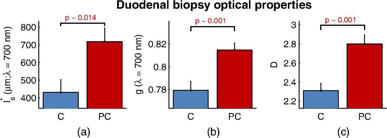
2.1.

Scattering Theory: Born Approximation in Continuous Random Media

In this section, we briefly review the application of the Born approximation in a continuous random media to calculate the scattering characteristics needed for the current study. Comprehensive discussion of scattering theory under the Born approximation can be found in Chapter 13 of Ref. 18, Chapter 7 of Ref. 19, and Chapter 6 of Ref. 20. A more specific treatment for continuous random media is found in Chapter 16 of Ref. 21. Application to biological tissue using the Whittle-Matérn family of autocorrelation functions was first presented in Refs. 22 and 23.

Scattering contrast within biological tissue is generated by the random arrangement of a number of arbitrarily shaped structures ranging in size from tens of nanometers to tens of microns.²⁴ The best way to mathematically describe such a randomly distributed media is through its statistical refractive index autocorrelation function $B_n(r_d)$. One versatile model to describe $B_n(r_d)$ uses the three-parameter Whittle-Matérn family of autocorrelation functions.^22–25

Fig. 1

Demonstration of the random media specified by the Whittle-Matérn model for (a) $D=2$, (b) $D=3$, and (c) $D=4$. The methods used to generate these images are described in Sec. 3.3.

In this paper, we refer to $A_n$, $L_n$, and $D$ as ultrastructural properties since they govern the spatial distribution of subdiffractional fluctuations in refractive index. Additionally, we refer to values of $r_d$ as structural length-scales (e.g., subdiffractional information is carried at short structural length-scales below $\sim \lambda /2$).

In order to relate $B_n(r_d)$ to light scattering, we apply the first Born approximation to calculate the power spectral density ${\mathrm{\Phi }}_s$ as the three-dimensional (3-D) Fourier transform of $B_n(r_d)$.²¹ For the Whittle-Matérn model, ${\mathrm{\Phi }}_s$ can be calculated analytically as²²

In order to describe the directionality of scattered light intensity, the differential scattering cross-section per unit volume for unpolarized light $\sigma (\theta )$ can be calculated by multiplying ${\mathrm{\Phi }}_s(k_s)$ by the dipole radiation pattern.

The shape of $\sigma (\theta )$ can be parametrized by the scattering mean free path $l_s$ (i.e., inverse of the scattering coefficient ${\mu }_s$) and the anisotropy factor $g$ (i.e., how forward directed the scattering is).²⁰

Finally, the effective transport for a diffusely scattering medium is expressed by the transport mean free path.

We refer to $l_s$, $g$, and $l_s^{*}$ as optical properties.

Analytical equations relating the ultrastructural and optical properties under the Whittle-Matérn model can be found in Ref. 22. One relationship that is useful to describe in further detail is that between $l_s^{*}$ and $D$. In the limit of $k{L}_n\gg 1$,

In words, this means that for $D<4$, the spectral dependence of $l_s^{*}$ follows a power-law distribution whose power is solely dependent on $D$. In this way, although $D$ should primarily be thought of as an ultrastructural property, it is also conceptually useful to think of it as an optical property that determines how strongly light transport changes with illumination wavelength.

2.2.

Enhanced Backscattering Theory

In this section, we briefly review the theoretical aspects of EBS that are pertinent to the discussion in the following sections. Additional details concerning the origin of EBS can be found in a number of seminal publications on the first experimental observation of EBS.^26–29 More recently, publications from our group detail the application of EBS to biological tissue characterization. These publications include an open source Monte Carlo program,³⁰ detailed description of the bench-top instrument used to measure biological tissue,⁷ description of the measurement of the spatial reflectance profile using EBS,¹¹ description of an inverse method to extract optical properties,³¹ and development of a miniaturized probe-based LEBS instrument to characterize tissue in vivo.¹⁴

The EBS signal is an angular intensity peak [$I_{\text{EBS}}({\theta }_x,{\theta }_y)$, see Fig. 2(a)] with its maximum value centered in the backscattering direction. The origin of $I_{\text{EBS}}({\theta }_x,{\theta }_y)$ is the constructive interference between all time-reversed path-pairs within a scattering medium. Mathematically, the interference signal from all path-pairs exiting the medium within the illumination spot can be summed using a Fourier transform operation to obtain the total observable signal.⁷

Fig. 2

Example data showing average measurements from all colorectal cancer (CRC) control biopsy samples. (a) measured at $\lambda =700\mathrm{nm}$. (b) Log-scale $P(x_s,y_s)$ obtained through inverse Fourier transform. The red arrows indicate inaccuracies in the measurement of $P(x_s,y_s)$ due to noise amplification as described in Sec. 3.1. (c) distribution obtained after integration over the azimuthal angle.

Of primary interest for tissue characterization is function $P(x_s,y_s)$, commonly known by a number of different names including spatially resolved diffuse reflectance,^32,33 spatial backscattering impulse-response,¹¹ diffuse reflectance profile, etc. While there are a great many instruments that measure some aspect of $P(x_s,y_s)$,^34–36 part of the power of using EBS is that it provides noncontact measurement of $P(x_s,y_s)$ at very short length scales ranging from $(y_s,x_s)=\pm 30\mu \text{m}$ to $\pm 2.7\mathrm{mm}$ with $\sim 4\mu \text{m}$ spatial resolution.¹¹ This range of length scales enables comprehensive characterization of $P(x_s,y_s)$ within both the subdiffusion ($\sqrt{x_s+y_s}<l_s^{*}$) and diffusion regimes, allowing for accurate extraction of all three ultrastructural and optical properties.

3.1.

EBS Instrument and Data Processing

Detailed description and schematics for our EBS instrument can be found in Refs. 7 and 13. In brief, broadband visible light from a supercontinuum laser source (SuperK Extreme EXW-6, NKT Photonics A/S, Birkerød, Denmark) is coupled into a single-mode fiber (Thorlabs, Newton, New Jersey; mode field diameter of 4.6 μm at 680 nm) and collimated to an $\sim 10\mathrm{mm}$ beam diameter. The beam then passes through a linear polarizer and an iris that reduces its diameter to 2 mm in size before being directed onto the biopsy. Light backscattered from the sample is then collected by a $50/50$ nonpolarizing antireflection coated plate beam splitter, passes through a linear polarizer to detect the copolarized channel, and is focused onto a CCD camera (PIXIS 1024B eXcelon, Princeton Instruments, Trenton, New Jersey) by a 100 mm focal length achromatic lens. A liquid crystal tunable filter (VariSpec, PerkinElmer, Waltham, Massachusetts) attached to the camera separates the light into its component wavelengths. This configuration detects angular backscattering of up to 7.5776 deg with 0.0074 deg resolution and wavelengths between 500 and 720 nm with a 20 nm filter bandwidth. After inverse Fourier transform, this provides a minimum spatial resolution of 3.78 μm (at $\lambda =500\mathrm{nm}$) and a maximum spatial range of 5.42 mm (at $\lambda =700\mathrm{nm}$).

To process the data, the biopsy measurement is first background subtracted and then normalized by the total unpolarized incoherent intensity measured from a reflectance standard (spectralon $>98\%$ reflectance, Ocean Optics, Dunedin, Florida). $I_{\text{EBS}}({\theta }_x,{\theta }_y)$ is then obtained by subtracting the incoherent baseline with a plane fit, using data from an annular ring that is $\sim 1.8\mathrm{deg}$ away from the peak maximum. An example of the peak shape measured from a rectal biopsy with illumination in the linear copolarized configuration is shown in Fig. 2(a).

The angular data are then converted to spatial coordinates through inversion of Eq. (8) to obtain^7,13,37

Figure 2(b) shows the $P(x_s,y_s)$ distribution extracted from the measurement of $I_{\text{EBS}}({\theta }_x,{\theta }_y)$ in Fig. 2(a).

As a way to average noise and make it easier to display experimental results, we integrate $P(x_s,y_s)$ over the azimuthal angle to obtain $P(r_s)$.

In words, $P(r_s)$ represents the total reflected intensity that exits the medium in the backscattering direction within an annulus of radius $r_s$. Figure 2(c) shows the $P(r_s)$ distribution calculated from $P(x_s,y_s)$ in Fig. 2(b). Matlab code performing the operations in Eqs. (9) to (11) are posted on our laboratory website.³⁸

We note that since function $S$ decays to 0 for $r_s>\varnothing$, the measurement of $P(r_s)$ is physically limited to length-scales smaller than $\varnothing$ (2 mm in our case). Moreover, division by the decaying function $S$ increasingly amplifies noise at increasing $r_s$, making the measurement inaccurate as $r_s\to \varnothing$ [indicated by red arrows in Fig. 2(b)]. As such, in this paper, we only plot the shape of $P(r_s)$ for length-scales in which function $S$ is $>5\%$. This occurs at $\sim 0.88\varnothing$, or, in our case 1760 μm.

3.2.

EBS Extraction of Ultrastructural and Optical Properties

Determination of the ultrastructural and optical properties of each biopsy sample is performed by fitting the shape of $P(r_s)$ to the Whittle-Matérn model. This process was first presented in Ref. 7. Briefly, a series of Monte Carlo simulations using the open source code detailed in Ref. 30 was performed in order to generate a library of $P(r_s)$ for $D=2.0$ to 4.0 in 0.1 steps, $g=0.70$ to 0.96 in 0.02 steps, and $r_s/l_s^{*}=0.004$ to 4 in 0.004 steps. Through use of multidimensional interpolation, we are able to rapidly generate $P(r_s)$ for arbitrary optical properties within the library bounds. In order to extract the three ultrastructural properties, we minimize the sum squared error between the experimentally measured and library-generated $P(r_s)·S(r_s)$ using a gradient search method in Matlab. We fit each curve over the values of $r_s$ for which we see a significant difference between case and control. To avoid the contribution of absorption, we fit the data using the wavelength range from 600 to 700 nm. Within this range, the contribution from absorption is $\sim 1\%$ that of scattering in the mucosa and is therefore negligible. The three ultrastructural properties can then be converted to optical properties at each wavelength using the analytical equations in Ref. 22.

It is important to make note of two assumptions/limitations inherent in our fitting routine. First, the Monte Carlo simulations are performed for the index matching case, and therefore assume that there is no refractive index contrast at the boundary. In order to account for this in our model, we use an empirically derived scaling factor to adjust the magnitude of the Monte Carlo simulated $P(r_s)$. Second, our model assumes a single slab geometry. As such, this technique is not capable of separating the contribution of layers with varying ultrastructural properties and instead provides measurement of the bulk optical properties within the slab.

3.3.

Generation of Random Medium Realizations

To generate a single 2-D realization of the random media specified by $B_n(r_d)$, the following steps can be followed: First, calculate the 2-D Fourier transform of $B_n(r_d)$ and take the square root. This specifies the distribution of spatial frequencies present in the medium. Second, multiply the resulting function by a 2-D Gaussian white noise signal with 0 mean and a variance of 1. This creates randomness within the spatial frequency domain. Finally, return to spatial coordinates by calculating the inverse 2-D Fourier transform and add the real and imaginary components. Microscopic resolution renderings can be made by multiplying the spatial frequency domain function by an area normalized top-hat function with radius $k·\mathrm{NA}$, where NA is the desired numerical aperture.

3.4.

Experimental Biopsy Measurement Procedure

Two to three pinch biopsies ($\sim 2$ to 3 mm diameter) were taken from subjects undergoing normal endoscopic screening procedures in accordance with the institutional review board at NorthShore University Healthsystems. Biopsies $<2\mathrm{mm}$ in diameter were not measured since they were smaller than the illumination beam diameter. For the CRC study, biopsies were collected from histologically normal sites within the rectal mucosa of subjects undergoing colonoscopy. Progression of field carcinogenesis was categorized according to the size of the largest adenomatous polyp found during colonoscopy and verified by a hospital pathologist. Four groups were assigned: healthy control (C, $N=43$) with no adenomatous polyps found during colonoscopy, diminutive adenomas (DA, $N=6$) with diameter $<5\mathrm{mm}$, adenomas (A, $N=25$) with diameter from 5 to 9 mm, and advanced adenomas (AA, $N=19$) with diameter $>10\mathrm{mm}$ or adenocarcinoma. For the PC study, biopsies were collected from histologically normal periampullary duodenum of subjects undergoing upper endoscopy procedures. Subjects were categorized into two groups: healthy controls (C, $N=13$) included individuals without any personal/family history of cancer or pancreato-biliary disease and the PC group ($N=19$) included subjects harboring adenocarcinomas.

Biopsies from all subjects were transported to Northwestern University in phosphate buffered saline (PBS) solution and measured within 4 h of extraction. A minimum of five spectral EBS measurements ($\lambda =500$ to 700 nm in 20 nm steps) were acquired from the epithelial side of each biopsy. To prepare the sample for measurement, it was placed in the center of a glass slide, oriented with the epithelium facing upward, and covered with PBS. Two 1-mm spacers were then placed on either side of the biopsy and then covered with a 165-μm glass cover-slip. This served to (1) ensure a uniform 1 mm thickness between all measurements, (2) maintain hydration for the experiment duration, and (3) direct the specular reflection away from the detector.

After measurement with EBS, the biopsies were fixed in 10% formalin for a minimum of 24 h. The samples were then embedded in paraffin wax and sectioned (5 μm) according to standard protocols. Slides were stained with hematoxylin and eosin and imaged using a $10\times$ microscope objective.

4.1.

$P(r_s)$ in Colorectal Cancer and Pancreatic Cancer

Figure 3 shows the changes in $P(r_s)$ attributable to CRC field carcinogenesis measured in ex vivo rectal biopsies. The general shape of $P(r_s)$ in these biopsies is a strongly decaying function of $r_s$ with $\sim 90\%$ of the intensity falling within the first 1000 μm shown in Fig. 3(a). Going from the curve for control subjects (C) to those harboring advanced adenomas (AA), there is a downward and inward shift of $P(r_s)$, indicated by the black arrow. The center and thickness of each curve indicate the mean and standard error, respectively. Performing a two-tailed student’s $t$-test at each $r_s$, we find a statistical significance for values of $r_s$ ranging from $\sim 150$ to $700\mu \text{m}$ [shown as the shaded gray region in Fig. 3(a)].

Fig. 3

CRC field carcinogenesis alterations measured in the shape of $P(r_s)$ from rectal biopsies. (a) Comparison between $P(r_s)$ for advanced adenomas (AA, diameter $>10\mathrm{mm}$ or adenocarcinoma) versus control (C) with the thickness of the curve indicating the standard error between measurements. The arrow indicates the direction of the change from AA to C and the gray shaded region indicates the values of $r_s$ for which the curves are significantly different. (b) Difference (AA − C) between the curves shown in panel (a). The dotted circle indicates $r_{s,\text{optimal}}$ (i.e., the location of the most significant effect) of the difference curve. (c) Normalized intensity at $r_{s,\text{optimal}}$ for groups at increasing risk of CRC. DA, diminutive adenomas with diameter from 0 to 4 mm and A, adenomas with diameter from 5 to 9 mm.

In order to better visualize the location and magnitude of these changes, Fig. 3(b) shows the difference between $P(r_s)$ for control and AA subjects. For smaller values of $r_s$, the effect increases in magnitude, consistent with the argument that the alterations associated with field carcinogenesis are most pronounced in the superficial mucosal layers.⁴ As a way to determine the $r_s$ location with the most significant changes, we find the location in which the p-value is minimized. This value ($r_{s,\text{optimal}}$) is found at 267 μm and indicated as the dotted circle in Fig. 3(b).

Finally, to demonstrate the magnitude of the effect during the early progression of CRC, Fig. 3(c) shows the normalized intensity value of $P(r_s)$ at $r_s=r_{s,\text{optimal}}$ for the four subject groups ordered in increasing aggressiveness from left to right. Consistent with Figs. 3(a) and 3(b), we see a progression toward a lower intensity as the polyp aggressiveness increases with a maximal 18% decrease between control and AA subject groups. This effect is statistically significant at the 5% level for nondiminutive adenomatous polyps (i.e., diameter $>=5\mathrm{mm}$), an observation that is consistent with the earlier ex vivo CRC study.⁹

We note that the comparable curves for DA and A subjects omitted from Figs. 3(a) and 3(b) follow the same progression as demonstrated in Fig. 3(c). However, for figure clarity these data were not shown.

We repeated the above analysis for the PC study. Figure 4 shows the changes in $P(r_s)$ attributable to PC field carcinogenesis measured in ex vivo duodenal biopsies. Going from the curve for control subjects to those with PC, there is a downward and inward shift of $P(r_s)$, similar to the trend observed in CRC. We find a statistical significance over values of $r_s$ ranging from $\sim 20$ to 900 μm. Figure 4(b) shows the difference between $P(r_s)$ for control and PC subjects. As $r_s$ approaches 0, we find a monotonically increasing effect with $r_{s,\text{optimal}}=20\mu \text{m}$. Finally, Fig. 4(c) shows the normalized intensity value of $P(r_s)$ at $r_s=r_{s,\text{optimal}}$ for control versus PC. This shows a 56% reduction in intensity from control to PC, which is statistically significant at the 5% level.

Fig. 4

Pancreatic cancer (PC) field carcinogenesis alterations measured in the shape of $P(r_s)$ from duodenal biopsies. (a) Comparison between $P(r_s)$ for PC versus control with the thickness of the curve indicating the standard error between measurements. The arrow indicates the direction of the change from PC to control and the gray shaded region indicates the values of $r_s$ for which the curves are significantly different. (b) Difference (PC − C) between the curves shown in panel (a). The dotted circle indicates $r_{s,\text{optimal}}$ of the difference curve. (c) Normalized intensity at $r_{s,\text{optimal}}$ for PC and control groups.

4.2.

Ultrastructural Alterations in CRC and PC

In order to gain a more physical understanding of the structural composition that leads to the observed alterations in $P(r_s)$, we extracted the ultrastructural properties from the shape of $P(r_s)$ as described in Sec. 3. We note that this extraction routine assumes that the medium is composed of a single slab of random media, which follows the Whittle-Matérn model. As such, the extracted values provide estimates for the bulk ultrastructural and optical properties over the entire biopsy.

Figure 5(a) shows the shape of $B_n(r_d)$ corresponding to the mean ultrastructural properties extracted for the control and AA subjects in the CRC study. The gray shaded region indicates the approximate range of structural length-scales over which EBS is sensitive to the shape of $B_n(r_d)$ ($\sim 30\mathrm{nm}$ to 3 μm).¹³ Interestingly, a reduction in the value of $B_n(r_d)$ is seen within the subdiffractional regime ($r_d<\lambda /2$, $\lambda =0.4\mu \text{m}$), but is negligible for structural length-scales within the resolution limit of a conventional imaging system. This implies that the alterations observed in the shape of $P(r_s)$ are primarily attributable to minuscule structures that could not be resolved in a conventional light microscope. To better convey this idea, Figs. 5(b) and 5(c) depict 1.4 NA microscope resolution renderings of the random media described by the shapes of $B_n(r_d)$ for control and AA subjects, respectively. In these images, all subdiffractional structures have been blurred away, leaving larger fluctuations that are qualitatively indistinguishable between control and AA subjects.

Fig. 5

Representations of the continuous random media extracted from the CRC study biopsy measurements. (a) $B_n(r_d)$ for control versus AA. The gray shaded region indicates the approximate range of values over which enhanced backscattering (EBS) is sensitive. (b) and (c) Continuous media realizations with 1.4 NA microscope resolution at $\lambda =0.4\mu \text{m}$ for the average ultrastructural properties of control and AA subjects, respectively. (d) and (e) Continuous media realizations over the EBS sensitivity range with the average ultrastructural properties of control and AA subjects, respectively.

In contrast with the microscope resolution images, Figs. 5(d) and 5(e) show renderings of the comparable random media with resolution (30 nm) and spatial extent (3 μm) chosen such that they match the structural length scale sensitivity of EBS. In this way, each rendering represents the range of structures that EBS “sees.” Comparison with the microscope resolution images demonstrates the sensitivity of EBS to much finer compositional details. Using this capability, it is possible to distinguish between control and AA subjects in Figs. 5(d) and 5(e), respectively. While the changes are very subtle, there is an appreciable reduction in the presence of smaller structural length-scales for AA subjects.

Repeating this analysis for the PC study, Fig. 6(a) shows the shape of $B_n(r_d)$ that corresponds to the mean ultrastructural properties extracted for all control and PC subjects. Similar to the CRC study above, a reduction in the value of $B_n(r_d)$ is seen within the subdiffractional regime, but becomes negligible almost exactly at the diffraction limit. This higher-frequency detail is almost entirely blurred away in the microscope resolution images in Figs. 6(b) and 6(c). Depictions of the range of structures detected by EBS for control and PC subjects are shown in Figs. 6(d) and 6(e), respectively. In this case, two prominent alterations are visible: (1) a reduction in refractive index variance and (2) a reduction in the presence of smaller structural length-scales.

Fig. 6

Representations of the continuous random media extracted from the PC study biopsy measurements. (a) $B_n(r_d)$ for control versus PC. The gray shaded region indicates the approximate range of values over which EBS is sensitive. (b) and (c) Continuous media realizations with 1.4 NA microscope resolution at $\lambda =0.4\mu \text{m}$ for the average ultrastructural properties of control and PC subjects, respectively. (d) and (e) Continuous media realizations over the EBS sensitivity range with the average ultrastructural properties of control and PC subjects, respectively.

4.3.

Optical Property Alterations in CRC and PC

To provide quantification of the measured field carcinogenesis changes in a way that is more comparable to other optical techniques, we convert the ultrastructural properties into optical properties using the analytical equations presented in Ref. 22. The values of $l_s^{*}$ measured at $\lambda =700\mathrm{nm}$, $g$ measured at $\lambda =700\mathrm{nm}$, and $D$ for CRC biopsies are shown in Fig. 7. We note that $D$ is included as an optical property in this plot since it demonstrates the spectral dependence of light transport (as described in Sec. 2). For all three optical properties, there is a statistically significant increase in value between C and AA subjects, with $l_s^{*}$ increasing 12.6%, $g$ increasing 1.9%, and $D$ increasing 5.1%.

Fig. 7

Optical properties of rectal biopsies in the CRC study. (a) $l_s^{*}$ measured at $\lambda =700\mathrm{nm}$. (b) $g$ measured at $\lambda =700\mathrm{nm}$. (c) Each plot shows $\text{mean}+\text{standard e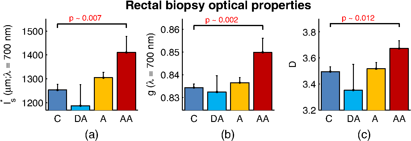rror}$. $N=43$ for C, $N=6$ for DA, $N=25$ for A, and $N=19$ for AA.

Following the progression from C to A to AA, there is a smooth increase in value for each optical property. While the DA values in our dataset do not follow this trend, the large standard error on their measurement (due to relatively small sample size) does not preclude the possibility of a smooth progression with larger sample size. Indeed, based on the trend in Fig. 4(c) and the compounding multistep nature of carcinogenesis, this is likely the case.

The optical properties for biopsies in the PC study are shown in Fig. 8. Once again, for all three optical properties, there is a statistically significant increase in value, with $l_s^{*}$ increasing 21.1%, $g$ increasing 4.6%, and $D$ increasing 66.9%. Interestingly, the directionality of the optical property changes in field carcinogenesis is the same for both CRC and PC.

Fig. 8

Optical properties of duodenal biopsies in the PC study. (a) $l_s^{*}$ measured at $\lambda =700\mathrm{nm}$. (b) $g$ measured at $\lambda =700\mathrm{nm}$. (c) Each plot shows $\text{mean}+\text{standard error}$. $N=13$ for C and $N=19$ for PC.

4.4.

Estimate of the Penetration Depth of Changes in CRC and PC

To obtain a better understanding of the depths at which the observed changes in $P(r_s)$ originate, we performed Monte Carlo simulations in which both $r_s$ and the maximum depth $z_{\max }$ of each photon were tracked to generate 2-D $P(r_s,z_{\max })$ distributions [shown in Figs. 9(a) and 10(a)]. Four simulations with optical properties corresponding to the mean values calculated for AA, CRC control, PC, and PC control were performed. For each simulation, a 2-D grid of $P(r_s,z_{\max })$ with fixed spatial coordinates corresponding to the experimentally measured range of values was initiated. Light intensity was then deposited into the fixed $P(r_s,z_{\max })$ grid positions until ${10}^{10}$ photon histories were computed.

Fig. 9

Penetration depth of in CRC field carcinogenesis using Monte Carlo simulation. (a) Log-scale $P(r_s,z_{\max })$ distribution for the average optical properties of all AA subjects. (b) Log-scale of the absolute difference in $P(r_s,z_{\max })$ between control and AA subjects. The dashed black line indicates $\overline{z_{\max }}(r_s)$. (c) Histological image from a rectal biopsy.

Fig. 10

Penetration depth of $P(r_s)$ in PC field carcinogenesis using Monte Carlo simulation. (a) Log-scale $P(r_s,z_{\max })$ distribution for the average optical properties of all PC subjects. (b) Log-scale of the absolute difference in $P(r_s,z_{\max })$ between control and PC subjects. The dashed black line indicates $\overline{z_{\max }}(r_s)$. (c) Histological image from a duodenal biopsy.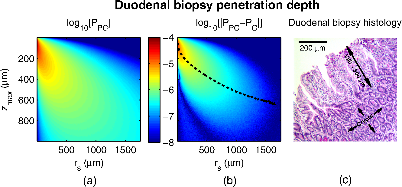

Figure 9 demonstrates the penetration depth of the $P(r_s)$ signal in CRC field carcinogenesis. The log-scale $P_{\mathrm{AA}}(r_s,z_{\max })$ distribution corresponding to the average optical properties of all AA subjects is shown in Fig. 9(a) ($P_C$ not shown since it is qualitatively very similar). As expected from multiply scattered light transport, with increasing values of $r_s$, there is a corresponding increase in $z_{\max }$. In order to isolate the location of the subtle differences in light propagation between control and AA subjects, Fig. 9(b) shows the absolute difference between $P_C(r_s,z_{\max })$ and $P_{\mathrm{AA}}(r_s,z_{\max })$ in log-scale. Qualitatively, the location of the changes with the largest magnitude is found at very small values of $r_s$ and $z_{\max }$. To better quantify the depth of these changes, we calculate the average penetration depth of the difference signal for each value of $r_s$ as

The values of $\overline{z_{\max }}(r_s)$ are represented as the dashed black line in Fig. 9(b).

Conceptually, $\overline{z_{\max }}$ represents the approximate depth at which the alterations occur (given the understanding that a wide range of depths do, in fact, contribute). Comparing with the values of $r_s$ for which the experimentally measured CRC $P(r_s)$ data are significantly separated [data shown in Fig. 3(a)], the depths at which the changes originate are between $\sim 400$ and 575 μm with the optimal difference occurring at 465 μm in depth. To qualitatively visualize the morphological structures interrogated over these depths, Fig. 9(c) shows a representative histological section acquired from one rectal biopsy. This image illustrates that the measured signal primarily originates from within the colonic crypts ($\sim 500\mu \text{m}$ in length) and surrounding extracellular matrix, which composes the superficial mucosal layer.

Figure 10 repeats the penetration depth analysis of the $P(r_s)$ signal for PC field carcinogenesis. The log-scale $P_{\mathrm{PC}}(r_s,z_{\max })$ distribution corresponding to the average optical properties of all PC subjects is shown in Fig. 10(a). Figure 10(b) shows the absolute difference between $P_C$ and $P_{\mathrm{AA}}$ in log-scale with the values of $\overline{z_{\max }}(r_s)$ represented as the dashed black line. Comparing with the values of $r_s$ for which the experimentally measured PC data are significantly separated [data shown in Fig. 4(a)], the depths at which the signal originates are between $\sim 100$ and 500 μm with the optimal difference occurring at 100 μm in depth. The representative histological section from one duodenal biopsy shown in Fig. 10(c) indicates that these depths correspond to the superficial mucosal layer, which is composed of villi, crypts, and the surrounding extracellular matrix.