Noise-equivalent sensitivity of photoacoustics

Amy M. Winkler; Konstantin I. Maslov; Lihong V. Wang

doi:10.1117/1.JBO.18.9.097003

11 September 2013 Noise-equivalent sensitivity of photoacoustics

Amy M. Winkler, Konstantin I. Maslov, Lihong V. Wang

Author Affiliations +

Journal of Biomedical Optics, Vol. 18, Issue 9, 097003 (September 2013). https://doi.org/10.1117/1.JBO.18.9.097003

Abstract

The fundamental limitations of photoacoustic microscopy for detecting optically absorbing molecules are investigated both theoretically and experimentally. We experimentally demonstrate noise-equivalent detection sensitivities of 160,000 methylene blue molecules (270 zeptomol or 2.7×10 ⁻¹⁹mol ) and 86,000 oxygenated hemoglobin molecules (140 zeptomol) using narrowband continuous-wave photoacoustics. The ultimate sensitivity of photoacoustics is fundamentally limited by thermal noise, which can present in the acoustic detection system as well as in the medium itself. Under the optimized conditions described herein and using commercially available detectors, photoacoustic microscopy can detect as few as 100s of oxygenated hemoglobin molecules. Realizable improvements to the detector may enable single molecule detection of select molecules.

1. Introduction

Photoacoustic tomography has been drawing the attention of the biomedical imaging community in the last decade.¹ A cross-over between optical imaging and ultrasound imaging, photoacoustics harnesses both the exquisite molecular contrast of optical absorption and the low scattering of ultrasound. Clinically, photoacoustic tomography is being used to add optical contrast to ultrasound imaging of breast cancer, due to its ability to image with acoustic resolution at depths beyond the optical diffusion limit, down to 2 cm demonstrated in vivo² and 8 cm in tissue phantoms,³ while retaining specific molecular sensitivity from optical absorption. Photoacoustics has also proven to be a highly scalable technique, achieving subcellular resolution within a millimeter depth of tissue.¹^,⁴^,⁵ Since the photoacoustic effect involves the transduction of light energy into sound energy, photoacoustic images are largely background free and present 100% sensitivity to optical absorption.⁶ The high imaging contrast of photoacoustics has enabled quantification of a number of vascular metrics, including total hemoglobin concentration ( $C_{Hb}$ ), blood oxygen saturation ( ${sO}_{2}$ ), flow speed or volumetric flow rate, capillary density, metabolic rate of oxygen ( ${MRO}_{2}$ ), and pulse wave velocity.⁷^,⁸ Furthermore, nonlinear effects have enabled ultrasharp spectroscopy⁹ and even subdiffraction imaging with spatial resolution $< 100 nm$ ,¹⁰ making photoacoustic imaging the only optical imaging technique to break through both the optical diffusion and optical diffraction limits. At the subdiffraction scale, however, the achievable resolution is limited by sensitivity as the number of molecules within a resolvable voxel becomes very small; e.g., a 10-nm cube contains only three hemoglobin molecules at the corpuscular concentration, i.e., the concentration within a red blood cell (RBC).

Recently, a number of absorption-sensitive optical techniques have achieved single molecule sensitivity at room temperature, including photothermal,¹¹ stimulated emission,¹² ground state depletion,¹³ and transmission microscopy.¹⁴ In this article, we discuss the challenges in achieving a similar sensitivity using photoacoustics and estimate the sensitivity with optimum illumination and state-of-the-art acoustic detectors to be between 10s and 1000s of molecules, depending on the molecule. By defining the optimum parameters for high molecular sensitivity, we outline the path toward expanding the scalability of photoacoustics further into this regime.

2. Theory

2.1.

Photoacoustic Signal

A photoacoustic signal is generated by intensity-modulated light in the frequency range of hundreds of kilohertz to a few gigahertz. The generated pressure amplitude is proportional to the modulated light intensity, which implies that the generated acoustic intensity is proportional to the square of the modulated light intensity. So in the sense of energy conversion, the photoacoustic effect is nonlinear. Pushing the sensitivity of photoacoustics then logically requires the use of high optical intensity; however, as in any optical excitation technique, photoacoustic generation exhibits nonlinearity in another sense due to optical absorption saturation, which prevents the pressure wave amplitude from increasing indefinitely with an optical intensity. Nonlinear thermal expansion of the medium with temperature can offset optical absorption saturation to some extent as it typically enhances photoacoustic generation. Furthermore, at very high optical intensities, heat can be deposited fast enough to generate shock waves. Here, we will not take into account thermal and acoustic nonlinear enhancements of photoacoustic generation because the temperature and pressure rises are small at the absorber concentrations considered. The following theoretical description seeks to determine the optimum parameters, such as optical intensity and modulation frequency, for photoacoustic generation from a small absorber, with the ultimate goal of detecting a single molecule.

The frequency domain solution for the pressure amplitude, $\tilde{p}$ , measured outside a small oscillating volume, such that the object size, $a$ , is much less than the acoustic wavelength, $λ$ , or $a ≪ λ$ , can be expressed as¹⁵

Eq. (1)

\tilde{p} (r, ω) = \frac{- i ω ρ}{4 π r} \tilde{Q} (ω) e^{i ω r / v_{s}},

where

r

is the distance from the center of the spherical absorber to the point of measurement,

ω

is the angular frequency,

v_{s}

is the speed of sound, and

\tilde{Q} (ω)

is the Fourier transform of the source-strength function,

Q (t)

. Physically,

Q (t)

is the rate of volume expansion of the object due to heat, such that

Q (t) = β H (t) / ρ C_{p}

, where

H (t)

is the absorbed optical power deposited in the form of heat inside the object,

ρ

is the mass density,

β

is the thermal expansion coefficient, and

C_{p}

is the specific heat. When

a ≪ λ

,

\tilde{p} (r, ω)

does not depend on the object shape but rather on the intrinsic properties

ρ

,

β

, and

C_{p}

. For most optically absorbing pigments, the molecular size is much smaller than the thermal diffusion length,

l_{t} = \sqrt{2 χ / ω}

, where

χ

is the thermal diffusivity of the medium (typically water), even up to a very high frequencies.¹⁶ In other words, heat diffuses into the surrounding medium within a single cycle and we can safely assume that almost all the volume expansion occurs within the surrounding medium and use

ρ

,

β

, and

C_{p}

of water in further calculations. Without further definition, tilde will be used to denote the frequency counterpart of the time-domain physical quantities, such as

H (t)

and

I (t)

.

In the linear case, $\tilde{H} (ω) = m σ \tilde{I} (ω)$ , where $m$ is the number of molecules, $σ$ is the optical absorption cross section, and $\tilde{I} (ω)$ is the Fourier transform of the optical intensity, $I (t)$ , and Eq. (1) becomes

Eq. (2)

\tilde{p} (r, ω) = \frac{- i β ω}{4 π C_{p} r} m σ \tilde{I} (ω) e^{i ω r / v_{s}} .

In Eq. (2), $\tilde{p} (r, ω)$ increases linearly with $\tilde{I} (ω)$ ; however, optical absorption saturation can induce significant nonlinearity for large $\tilde{I} (ω)$ . On average, the optical power absorbed by a single molecule, $H_{SM}$ , is of the form¹⁷

Eq. (3)

H_{SM} = \frac{σ I}{1 + b I / I_{sat}} .

Here, $b$ is a value between 1 and 2 depending on the electronic states of the molecule ( $b \approx 2$ for a two-level system and $b \approx 1$ for a three-level system) and $I_{sat}$ is the saturation intensity of the molecule equal to $h ν / (σ τ)$ , where $h$ is the Planck’s constant, $ν$ is the optical frequency, and $τ$ is the relaxation time. As $I$ approaches $I_{sat}$ , $H_{SM}$ increases significant nonlinearly, approaching a finite value as $I$ tends to infinity.

To extend the analysis of the photoacoustic signal to the nonlinear regime, the Fourier transform of $H_{SM}$ , is substituted for $σ \tilde{I}$ in Eq. (2)

Eq. (4)

\tilde{p} (r, ω) = \frac{- i β ω}{4 π C_{p} r} m {\tilde{H}}_{SM} (ω) e^{i ω r / v_{s}}, n \geq 1 .

For sinusoidal excitation, i.e.,

Eq. (5)

I (t) = I_{0} [1 + \cos (ω_{o} t)],

optical absorption saturation induces periodic heat deposition at harmonics of

ω_{0}

. The amplitudes are computed by substituting Eqs. (5) into (3) and performing a Fourier cosine transformation, as shown in Eq. (6):

Eq. (6)

{\tilde{H}}_{n} = \frac{ω_{o}}{π} \int_{- π / ω_{o}}^{π / ω_{o}} {\frac{σ I_{0} [1 + \cos (ω_{o} t)]}{1 + b I_{0} [1 + \cos (ω_{o} t)] / I_{sat}}} \cos (n ω_{o} t) d t = \frac{2 σ b^{- 1} I_{sat}}{\sqrt{1 + 2 b I_{0} / I_{sat}}} {[\frac{\sqrt{1 + 2 b I_{0} / I_{sat}} - (1 + b I_{0} / I_{sat})}{b I_{0} / I_{sat}}]}^{n}, n \geq 1,

where the closed form solution to the integration can be found in Ref. 18. The complex amplitudes

{\tilde{p}}_{n}

of photoacoustically induced pressure waves at harmonics of

ω_{o}

are expressed by substituting

{\tilde{H}}_{n}

in for

{\tilde{H}}_{SM} (ω)

in Eq. (4):

Eq. (7)

{\tilde{p}}_{n} (r) = \frac{- i β n ω_{o}}{4 π C_{p} r} m {\tilde{H}}_{n} e^{i n ω_{o} r / v_{s}}, n \geq 1 .

{\tilde{H}}_{n}

and

{\tilde{p}}_{n} (r)

as a function of

b I_{0} / I_{sat}

are shown in Fig. 1 for

n = 1

, 2, 3, and 4.

{\tilde{H}}_{n}

and

{\tilde{p}}_{n} (r)

reach finite maxima at the same

I_{0}

for each harmonic.

{\tilde{H}}_{n}

is highest at the fundamental frequency, i.e.,

n = 1

; however, the linear dependence of

{\tilde{p}}_{n} (r)

on

n

causes the maximum

{\tilde{p}}_{n} (r)

to increase for higher harmonics.

Fig. 1

Fourier coefficients of the (a) absorbed optical power, $| {\tilde{H}}_{n} |$ , and (b) pressure amplitude, $| {\tilde{p}}_{n} |$ , and peak values of the total (c) pressure, and (d) acoustic intensity in the time domain as a function of an optical intensity. The peaks of the absorbed optical power and pressure occur at the same optical intensity values. The absorbed optical power is highest at the fundamental frequency, regardless of the intensity, while the frequency component that generates the highest pressure amplitude varies with intensity. As expected, the peak pressure of the summation of all frequency components saturates with an optical intensity. The acoustic intensity follows the square of the saturation curve.

The optimum $I_{0}$ , determined as a function of $n$ by setting the first derivative of ${\tilde{H}}_{n}$ with respect to $I_{0}$ equal to 0, is given by

Eq. (8)

I_{0}^{opt} (n) = n (n + \sqrt{1 + n^{2}}) b^{- 1} I_{sat},

where

I_{0}^{opt}

is the optimum

I_{0}

.

As $n \to \infty$ , the peak of ${\tilde{p}}_{n} (r)$ approaches a finite value. Increasing from $n = 1$ to $n \to \infty$ only improves the signal by $1.07 \times$ , while the system cost and complexity increase significantly with $n$ . Therefore, detection at the fundamental frequency is preferred.

Reaching the optimum modulated optical intensity value at the fundamental frequency, $I_{0}^{opt} (n = 1) = (1 + \sqrt{2}) b^{- 1} I_{sat} \approx 2.4 b^{- 1} I_{sat}$ , is possible for many target molecules by using high power continuous-wave lasers (typically 5 to 10 W) and high numerical aperture (NA) optics. For example, the saturation intensity of oxygenated hemoglobin in the Q-band of the absorption spectrum is $100 MW / {cm}^{2}$ .¹⁹ In the case of a Gaussian beam profile, a peak intensity of $500 MW / {cm}^{2}$ can be achieved with 2 W incident power with beam waist 0.5 μm, achievable with commercially available continuous-wave lasers and objective lenses. Inserting $n = 1$ , $I_{0} = (1 + \sqrt{2}) b^{- 1} I_{sat}$ , and $I_{sat} = h ν / σ τ$ into Eqs. (6) and (7) gives

Eq. (9)

{\tilde{p}}_{1} (r) = \frac{- i (3 - 2 \sqrt{2}) β ω_{o} m h ν}{2 π C_{p} τ b} (\frac{e^{i ω_{o} r / v_{s}}}{r}) .

This form of the pressure wave amplitude from a small absorber reveals that molecules with shorter relaxation times can generate higher signals, provided $I_{0} = (1 + \sqrt{2}) b^{- 1} I_{sat}$ can be achieved at focus.

Finally, we consider the effect of acoustic attenuation in the acoustic coupling medium. Inserting the acoustic attenuation term into Eq. (9) reveals that the optimum frequency depends upon the acoustic attenuation constant, $α$ , and distance, $r$ :

Eq. (10)

{\tilde{p}}_{1} (r) = \frac{- i (3 - 2 \sqrt{2}) β ω_{o} m h ν}{2 π C_{p} τ b} \frac{e^{i ω_{o} r / v_{s}}}{r} e^{- α {(ω_{o} / 2 π)}^{2} r} .

For example, at a distance of 6 mm in water, which has $α = 25 \times 10^{- 15} {Hz}^{- 2} m^{- 1}$ , the optimum frequency is approximately 60 MHz. Here, we consider a quadratic dependence on $r$ , which is applicable to water and other homogeneous fluids. For tissue, which comprises multiple acoustically absorbing components, the dependence on $r$ is approximately linear.

2.2.

Noise

Noise in photoacoustics arises from the medium as well as the detector. The medium exhibits thermal acoustic noise that fundamentally limits the detection of any photoacoustic signal.²⁰^,²¹ The power spectral density of acoustic thermal noise is $k_{B} T$ which equates to a power spectral density on a detector with efficiency $η$ of²¹

Eq. (11)

N_{a} (f) = η (f) k_{B} T,

where

η (f)

is the detector efficiency at frequency,

f

, defined as the fraction of acoustic power converted into electrical power,

k_{B}

is the Boltzmann constant, and

T

is the absolute temperature of the medium. (Compared to the notation used by Rhyne²¹

η = {| G_{r} |}^{2} Z_{a} / (A R)

, where

G_{r}

is the ratio between detector voltage and incident pressure,

Z_{a}

is the characteristic acoustic impedance of the medium,

A

is the detector area, and

R

is the active (real) part of the detector electrical impedance.)

Acoustic detectors also generate their own noise. For piezoelectric transducers, thermal noise is generated from the transducer active element backing and electrical and mechanical losses in transducer. This noise is modeled as a Johnson noise source associated with the active (real) part of the internal impedance of the transducer. By adding electronic components inside the transducer package, a 50 Ω impedance is typically achieved over its bandwidth. Here, we consider a piezoelectric transducer with an internal resistance matched to a receiver (i.e., preamplifier) with load resistance $R$ . In this case, the power spectral density of thermal noise from the transducer’s internal resistance across the load resistor is given by²¹

Eq. (12)

N_{d} (f) = k_{B} T .

The preamplifier introduces additional noise. With a matched impedance, the preamplifier noise is well described by its noise factor, $F_{n}$ , which is the ratio of noise at the output of the preamplifier to the thermal noise of the source resistor. The power spectral density of noise added by the preamplifier with a given $F_{n}$ is²²

Eq. (13)

N_{p} (f) = N_{d} (f) (F_{n} - 1) .

Acoustic detector sensitivity is quantified by the noise equivalent pressure (NEP), which can be expressed as a spectral density with units of $P a / \sqrt{Hz}$ . The $NEP (f)$ is derived from the sum of the noise power spectral densities in Eqs. (11)–(13) as follows:

Eq. (14)

NEP (f) = \sqrt{k_{B} T [1 + F_{n} / η (f)] Z_{a} / A} .

The detector parameters that influence $NEP (f)$ are $F_{n}$ , $η$ , and $A$ . Low-noise preamplifiers typically exhibit $F_{n} \approx 2$ . Resonant transducers, such as those used in high-intensity focused ultrasound (HIFU) applications, can readily achieve on-resonant efficiencies, $η$ , of 0.5 ( $- 3 dB$ ) or better, and in this case, the noise contributions from the medium and detector are within the same order of magnitude.²³ For a spherically focused transducer with $r = 6 mm$ and NA 0.5, corresponding to $A \approx 30 {mm}^{2}$ in room temperature ( $T = 300 K$ ) water with $Z_{a} \approx 1.5 \times 10^{6} Rayls / m^{2}$ , the $NEP (f)$ can be around $30 μ Pa / \sqrt{Hz}$ .

For broadband detectors, however, $η (f) ≪ 1$ ; hence, detector noises dominate. As a result, Eq. (14) simplifies to

Eq. (15)

NEP (f) = \sqrt{F_{n} k_{B} T Z_{a} / [A η (f)]} .

Typical broadband transducers have $η (f)$ between 0.01 ( $- 20 dB$ ) and 0.001 ( $- 30 dB$ ) with area typically around $30 {mm}^{2}$ . Again, if $F_{n} \approx 2$ , the $NEP (f)$ is in the range of 0.2 to $0.6 mPa / \sqrt{Hz}$ . By comparison, optical detection schemes are approaching the sensitivity of broadband piezoelectric transducers with reported values as sensitive as $2.0 mPa / \sqrt{Hz}$ .²⁴

The number of molecules required to generate photoacoustic pressure equal to NEP is the noise equivalent number of molecules (NEM). To compute the NEM, the noise standard deviation is divided by the signal from a single molecule. In terms of variance and signal power, the NEM is equal to the square root of the variance, i.e., noise power, divided by the square root of the signal power from a single molecule. Within a bandwidth, $Δ f$ , narrow compared to the transducer bandwidth such that $η (f) \approx η (f_{o})$ , the NEM is given by

Eq. (16)

NEM = \sqrt{F_{n} k_{B} T Δ f / [η (f_{o}) S_{SM} (f_{o})]},

where

S_{SM} (f_{o})

is the photoacoustic power from a single molecule at the fundamental frequency,

f_{o}

. NEM increases with

Δ f

, which for the case of modulated continuous-wave photoacoustics (CW-PA) directly relates to integration time

Δ t

by

Δ f = 1 / (2 Δ t)

.

Under the optimum intensity-modulated illumination conditions described in Sec. 2.1 and summarized in Eq. (10), the power from a single molecule ( $m = 1$ ) at $f_{o}$ is given by

Eq. (17)

S_{SM} (f_{o}) = \frac{{| {\tilde{p}}_{1} (r; m = 1) |}^{2} A}{2 Z_{a}} = \frac{2 π {[β f_{o} (3 - 2 \sqrt{2})]}^{2}}{Z_{a} C_{p}^{2}} {(\frac{h ν}{τ b})}^{2} \frac{A}{4 π r^{2}} e^{- 2 α f_{o}^{2} r} .

S_{SM} (f_{o})

, here, is given for a spherical wave and is proportional to

A

and inversely proportional to

r^{2}

. However, the total area for a sphere is

4 π r^{2}

, so the power over

4 π

solid angle is conserved. The fraction of power at the detector is

A / (4 π r^{2})

, which is proportional to the square of the NA for small angles,

A / (4 π r^{2}) = [1 - \sqrt{1 - {NA}^{2})}] / 2 \approx {NA}^{2} / 4

. The highest sensitivity for a small absorber, therefore, is achieved by maximizing both NA and

ω_{o}

while minimizing

r

.

To separately consider generation and detection effects, we split the denominator of Eq. (16) into two parameters, photoacoustic power generated by a single molecule before propagation, $S_{g} (f_{o})$ (W), and transmission loss, $T_{d} (f_{o})$ (dimensionless), which includes acoustic propagation, acoustic attenuation, and transduction loss, such that

Eq. (18)

η (f_{o}) S_{SM} (f_{o}) = S_{g} (f_{o}) T_{d} (f_{o}),

S_{g} (f_{o}) = \frac{2 π {[β f_{o} (3 - 2 \sqrt{2})]}^{2}}{Z_{a} C_{p}^{2}} {(\frac{h ν}{τ b})}^{2},

T_{d} (f_{o}) = η (f_{o}) \frac{{NA}^{2}}{4} e^{- 2 α f_{0}^{2} r} .

Transmission loss depends on several transducer parameters: efficiency $η (f_{o})$ , NA, and focal length $r$ . A table of some commercially available transducers is shown in Table 1. A more comprehensive list of transducer materials and properties as well as the ultimate sensitivities of transducers used in broadband detection mode is available in Ref. 25. The listed transducers, all with similar NAs, have center frequencies from 2.45 to 200 MHz. Low loss ( $η \approx - 3 dB$ ), resonant transducers have bowl-shaped, air-backed active elements with thicknesses around $λ / 2$ at the resonant frequency and are made from high efficiency Pz27 piezoceramic. At high frequencies, the piezoelectric element is a crystal (typically ${LiNbO}_{3}$ ) or vacuum-deposited texture (ZnO) that cannot have high curvature. Therefore, it is placed onto a solid buffer element, such as a fused quartz or sapphire piece, which can be ground into an acoustic lens. An anti-reflection coating can then be deposited onto the buffer/lens element. The lens arrangement plus diffraction effects typically exhibit losses of $- 4 dB$ . At the resonant frequency, the piezoelectric transducer can have losses as low as $- 3 dB$ for longitudinal waves,²⁶ totaling $- 7 dB$ for the entire transducer.²⁷ Current commercially available transducers for high frequencies, however, are optimized for a broadband and use an impedance matched, sound absorbing backing. This backing damps the transducer and introduces higher losses ( $η \approx - 20 dB$ ). Electro-mechanical coupling between the transducer output and backing also introduces an active component to the transducer’s electrical impedance and is a major source of thermal noise.

Table 1

Estimated transducer sensitivity.

Vendor	Numerical aperture	$f$ (MHz)	$η$ (dB)	Focal length in water, $r$ (mm)	Area, $A$ ( ${mm}^{2}$ )	NEP ( $Pa / \sqrt Hz$ )	$T_{d}$	$S_{g}$ (W)		NEM ( $1 / \sqrt Hz$ )
Vendor	Numerical aperture	$f$ (MHz)	$η$ (dB)	Focal length in water, $r$ (mm)	Area, $A$ ( ${mm}^{2}$ )	NEP ( $Pa / \sqrt Hz$ )	$T_{d}$	${HbO}_{2}$	MB	${HbO}_{2}$	MB
FerroPerm Piezoceramic, Kristgaard, Denmark	0.85	2.45	$- 3$	22	1439	$4.6 \times 10^{- 6}$	0.12	$2.1 \times 10^{- 24}$	$7.1 \times 10^{- 27}$	204	3522
FerroPerm Piezoceramic, Kristgaard, Denmark	0.83	5	$- 3$	12	405	$8.8 \times 10^{- 6}$	0.11	$8.8 \times 10^{- 24}$	$3.0 \times 10^{- 26}$	103	1783
Olympus NDT Panametrics	0.50	50	$- 20$	6	30	$2.0 \times 10^{- 4}$	$3.2 \times 10^{- 4}$	$8.8 \times 10^{- 22}$	$3.0 \times 10^{- 24}$	173	2982
Olympus NDT Panametrics	0.80	125	$- 30$	2	10	$1.1 \times 10^{- 3}$	$4.2 \times 10^{- 5}$	$5.5 \times 10^{- 21}$	$1.8 \times 10^{- 23}$	189	3270
Kibero GmbH, Saarbrücken, Germany	0.87	200	$- 30$	1	3	$2.0 \times 10^{- 3}$	$3.4 \times 10^{- 5}$	$1.4 \times 10^{- 20}$	$4.7 \times 10^{- 23}$	132	2275

The focal lengths of these transducers tend to decrease with frequency, since frequency-dependent acoustic attenuation limits the usable path length in water. A more thorough analysis of the effect of acoustic attenuation in water on photoacoustic bandwidth can be found in Ref. 28. The transducer area similarly decreases with frequency, resulting in a similar NA for all the transducers.

The NEP depends on detection parameters $F_{n}$ , $η$ , and $A$ only and so the low frequency, resonant transducers are more sensitive by this metric. A preamplifier $F_{n}$ of 2 is assumed for all the transducers. The dimensionless transmittance, $T_{d}$ , depends on $η$ , NA (which includes $A$ and $r$ ), and acoustic attenuation and so the low frequency, resonant transducers are also more sensitive by this metric. Photoacoustic generation, however, increases with frequency, ultimately offsetting the lower detector sensitivities such that the NEM is of the same order of magnitude for all the transducers listed. The NEM is given for oxygenated hemoglobin and methylene blue with lifetimes of 22 ps¹⁹and 380 ps,²⁹ respectively, near $λ = 532 nm$ . The factor $b$ is set equal to 1.

3. Experimental Setup

3.1.

Photoacoustic System

To quantify the molecular sensitivity of photoacoustics per square root Hertz, we built an intensity modulated, CW-PA system. For media with dense absorbers, such as tissue, CW-PA imaging has been shown to be less sensitive than pulsed-PA imaging when the laser light intensity and pulse fluence are limited by the thermal damage threshold for tissue.³⁰^,³¹ The large increase of average temperature compared to pulsed-PA excitation can be problematic; however, the average temperature rise from low concentrations of absorbing molecules as we will show, is relatively small and unlikely to cause thermal damage. By tight focusing, CW lasers can achieve intensities beyond the saturation intensity of many types of molecules, and are thus capable of achieving the optimum intensity for a given molecule. Furthermore, CW-PA facilitates narrowband filtering for minimizing thermal noise.

A system diagram is shown in Fig. 2. The light source is a 532 nm CW laser (Spectra-Physics Millennia V, Newport, Irvine, CA) modulated by an electro-optic modulator (Model 350-105-01-RP, ConOptics, Inc., Danbury, CT). The electro-optic modulator is driven by a high-power amplifier (Model ZHL-100W-GAN+, Mini-Circuits, Brooklyn, NY) and DC bias supply (Model BPS1, ConOptics, Inc., Danbury, CT). Light is focused by a microscope objective with NA 0.4. The incident Gaussian beam is focused by the objective to a 1.4 μm waist. Light focuses at the sample mounted on a thin cover glass, which introduces negligible optical aberrations. The optical peak power at the sample was approximately 400 mW. The sample is acoustically coupled with deionized water to a plastic membrane, which forms the base of a custom-built water bath. The acoustic detector is a 50 MHz piezoelectric transducer (Model V214-BB-RM, Olympus NDT, Waltham, MA) with NA 0.5 and focal length of 6 mm (listed as the third item in Table 1). The electrical signal is amplified and sent to a lock-in amplifier (SR844, Stanford Research Systems, Sunnyvale, CA). The signal amplitude output of the lock-in amplifier was digitized with a data acquisition card (NI PCI 6251, National Instruments) and collected using a LabView interface (National Instruments). The root-mean-square noise in the system within a 1.25 Hz bandwidth was around 1 μV after 60 dB gain. Signals from the samples described herein ranged from 10s to 100s of μV.

Fig. 2

Narrowband continuous-wave photoacoustic (CW-PA) system. EOM, electro-optic modulator; Osc, oscilloscope; LIA, lock-in amplifier.

For validation, we also used a pulsed-PA system described previously.³² Briefly, an Nd:YVO4 pulsed laser (Elforlight, SPOT) generates 1.5 ns pulses at 532 nm. Light is focused onto the sample by an NA 0.1 objective. The acoustic detector is a 50 MHz piezoelectric transducer (Model V214-BB-RM, Olympus NDT, Waltham, MA), the same model as in the CW-PA system.

3.2.

Transducer Calibration

The transducer efficiency, $η$ , was deduced from pulse-echo measurements from a flat BK7 glass piece in water, with acoustic reflectivity, Refl, of 61%. The transducer was driven by 4 μs tone bursts through a 50 Ω source resistor with center frequencies varied from 5 to 80 MHz in 5 MHz increments. Both the initial pulse and received echo signal on a 50 Ω load were detected at an oscilloscope. The relationship between $η$ and the pulse-echo ratio, ${\tilde{V}}_{out} / {\tilde{V}}_{in}$ , was determined using the transducer model presented by Rhyne.²¹ Briefly, the transmitted pressure amplitude, ${\tilde{p}}_{t}$ , is equal to the conversion parameter, $G_{t}$ , times the driving (input) voltage ${\tilde{V}}_{in}$ . The reflected pressure, $\tilde{p}$ , at the transducer is equal to $\sqrt{Refl} \times {\tilde{p}}_{t}$ . The detected (output) voltage ${\tilde{V}}_{out}$ is equal to the conversion parameter $G_{r}$ times the pressure at the transducer, $\tilde{p}$ . For a reciprocal system, which is a valid assumption in our case as the transmitter and receiver impedances are the same, the conversion parameters $G_{t}$ and $G_{r}$ are related by the electrical and acoustic impedances as, $G_{t} = G_{r} Z_{a} / (2 RA)$ .²¹ Therefore,

Eq. (19)

{\tilde{V}}_{out} / {\tilde{V}}_{in} = \sqrt{Refl} \cdot {| G_{r} |}^{2} Z_{a} / (2 RA) .

The amplitude conversion $G_{r} = {\tilde{V}}_{out} / \tilde{p}$ is related to $η$ , which is the electric power spectral density, $S_{e}$ divided by the acoustic power spectral density, $S_{a}$ , such that $| G_{r} | = \sqrt{η (f) RA / Z_{a}}$ . Substituting into Eq. (19) results in an expression for $η$

Eq. (20)

η (f) = \frac{2 {\tilde{V}}_{out} (f)}{{\tilde{V}}_{in} (f) \sqrt{Refl}} .

The transducer efficiency, $η (f)$ , as well as the conversation factor between voltage and pressure on a 50 Ω load, $| {\tilde{V}}_{out} (f) | / | \tilde{p} (f) |$ , is plotted as a function of frequency in Fig. 3. The error bars are derived from the variation in detected voltage. The peak response is between 35 and 45 MHz with around 20 dB losses and $3 μ V / Pa$ conversion. Photoacoustic measurements later revealed 42 MHz to be the optimum operating frequency.

Fig. 3

Transducer calibration. (a) The transducer efficiency, $η$ in decibels, as a function of frequency. (b) The conversion factor between incident pressure and induced voltage in $μ V / Pascal$ as a function of frequency.

3.3.

Samples

Molecular sensitivity was quantified for two common targets in photoacoustic imaging—methylene blue and hemoglobin. To restrict the number of illuminated molecules, methylene blue dye (NDC 0517-0310-10, American Regent, Inc., Shirley, NY) was mixed with gelatin and molded to a known thickness. The mold consisted of two parallel strips of plastic shim stock, 12.7-μm thick (PL5-0005, Maudlin & Son Mfg Co. Inc., Houston, TX). A thin layer of glue was applied to the strips to fix them to a cover glass. Minute drops of methylene blue gel were placed between the strips and a second cover glass was used to confine the gel in the mold. Pulsed-PA imaging was used to measure the final thickness of the sample. Regions measured to be $< 30 - μ m$ thick (i.e., less than the acoustic wavelength) were used to estimate system sensitivity.

The number of illuminated hemoglobin molecules was restricted within a monolayer of RBCs, approximately 2-μm thick. Whole oxygenated bovine blood (Sigma–Aldrich, St. Louis, MO) was dropped onto a cover glass and spread into a monolayer. The RBCs were fixed to the cover glass by soaking in methanol for 30 min. The RBC monolayer was verified by bright field microscopy and CW-PA imaging.

The number of illuminated molecules was estimated by multiplying the number density of molecules by the illuminated volume within the sample, assuming the focus was placed at the center of the sample. For the methylene blue sample, the number of molecules per cubic micrometer was $1.88 \times 10^{6}$ , $1.88 \times 10^{5}$ , and $1.88 \times 10^{4} {μ m}^{- 3}$ for 0.1%, 0.01%, and 0.001% solutions, respectively. For hemoglobin, the average corpuscular hemoglobin concentration of 5.2 mM was assumed, which is equivalent to $3.1 \times 10^{6} {μ m}^{- 3}$ . The boundary of the illuminated volume was set at the $1 / e^{2}$ point assuming Gaussian beam propagation from the waist, which was 1.4 μm in the CW-PA system and 2.9 μm in the pulsed-PA system. In the CW-PA system, the illuminated volume was less than $< 243 {μ m}^{3}$ within the methylene blue sample ( $< 30 - μ m$ thick) and $12 {μ m}^{3}$ within the RBC monolayer (2-μm thick). Therefore, the number of illuminated molecules was $< 4.5 \times 10^{8}$ , $4.5 \times 10^{7}$ , and $4.5 \times 10^{6}$ for the methylene blue samples and $3.8 \times 10^{7}$ for the hemoglobin sample. In the pulsed-PA detection, the illuminated volume was $< 806 {μ m}^{3}$ within the methylene blue sample, corresponding to $1.5 \times 10^{9}$ , $1.5 \times 10^{8}$ , and $1.5 \times 10^{7}$ illuminated molecules for the methylene blue samples.

3.4.

Signal to Noise Measurements

Signal and noise measurements were taken for both samples. The signal-to-noise ratio (SNR) was calculated as the average signal over time (CW-PA detection only) and/or lateral position (both CW-PA and pulsed-PA detection) divided by the standard deviation of the background. NEM was calculated as the number of illuminated molecules divided by the SNR. The modulation frequency was optimized during the measurements and ultimately set at 42 MHz. Tone burst illumination with duty cycle $< 50 %$ ensured that the driving signal was “off” while the sample signal was received by the transducer. This precaution removed the possibility of electromagnetic coupling from the EOM driving signal to the sample signal within the detection bandwidth. The repetition rate was 83.33 kHz (period 12 μs), to accommodate the 6 μs delay time from the focus to the transducer. The duty cycle was adjusted during measurements for a given optical intensity to minimize thermal damage and nonlinearity. The lock-in amplifier bandwidth was set at 1.25 Hz, and the signal was measured for 5 to 10 s. Noise was quantified as the standard deviation of the signal when the laser was blocked. (Noise measurements were also taken in the absence of the sample with the laser unblocked, but the difference was insignificant.)

A risk in extrapolating to NEM using a sample with a higher number of molecules is that the signal may not scale proportionally due to thermal effects. The thermal expansion coefficient, $β$ , increases with temperature, causing the pressure amplitude to increase nonlinearly with absorbed optical power, $H$ . Unlike optical absorption saturation, which causes the increase in pressure amplitude to taper off with $H$ , thermal effects can cause the pressure amplitude to increase faster than the predicted rate. This increase could artificially improve our linearly extrapolated NEM. Therefore, to test for thermal nonlinear effects, the optical intensity was varied from the maximum intensity to approximately 10% of the maximum intensity using a variable attenuator. The maximum intensity in these studies was $< 4 %$ of the saturation intensity, so only thermal nonlinearity was considered a concern. A linear change in signal with an optical intensity then would indicate a negligible influence of thermal nonlinearity.

For the methylene blue sample, the SNR was measured using both the CW-PA and pulsed-PA systems, utilizing the same Panametrics transducer model for both systems. The pulsed-PA system operated much faster, due to its larger bandwidth, so it was used to scan the sample and estimate the variation in number of illuminated molecules due to sample heterogeneity. To minimize the average temperature rise during CW-PA imaging, the duty cycle was decreased to 10%. The effect of a partial duty cycle on the lock-in amplifier was tested using a 42 MHz tone burst signal from a function generator with 83.33 kHz repetition rate, while varying the duty cycle. The detected signal at the lock-in amplifier increased linearly with duty cycle from 10% to 100%, so we expect the extrapolated NEM to improve linearly with increased duty cycle.

The SNR of the RBC sample was measured using the CW-PA system with the same parameters. In the course of collecting data from this sample, which has a fixed concentration, we discovered the need to scan the sample back and forth by a few micrometers on a translation stage to dissipate heat. Again, to test for thermal nonlinear effects, which could result in erroneous estimation of the NEM, the optical intensity was varied from the maximum intensity ( $< 3 %$ of the saturation intensity) to approximately 10% of the maximum intensity using a variable attenuator.

3.5.

Imaging

The RBC sample was imaged using the CW-PA system. By imaging, various aspects of the system and sample could be checked simultaneously, such as the effect of electromagnetic coupling and the focal alignment. The lock-in amplifier bandwidth was increased from 1.25 to 780 Hz in order to image a $100 \times 100 pixel$ field of view within a few minutes. The illumination was adjusted to 100% duty cycle for imaging. While electromagnetic coupling was a concern at 100% duty cycle, any coupling would be evident in the images, so the risk of over or underestimating the system sensitivity due to coupling was small. Since, thermal damage was a concern at 100% duty cycle, the intensity was decreased to $730 kW / {cm}^{2}$ .

System parameters for each measurement are summarized in Table 2. The intensity values are given in units of $MW / {cm}^{2}$ and as a percentage of the molecules’ saturation intensities. At 532 nm, the saturation intensity is $70 MW / {cm}^{2}$ for methylene blue and $100 MW / {cm}^{2}$ for oxygenated hemoglobin.

Table 2

Parameters for each sample/photoacoustic system.

Molecule, imaging mode	Beam waist (μm)	Pulse or burst energy	Average power	Average intensity per illuminated volume per pulse or burst	Number of illuminated molecules	Duty cycle, %
Methylene blue, pulsed-PA	2.9	44 nJ	44 μW	$29 MW / {cm}^{2} = 41 %$ $I_{sat}$	$1.5 \times 10^{7}$ to $1.5 \times 10^{9}$	N/A
Methylene blue, CW-PA	1.4	21.6 to 240 mJ	1.8 to 20 mW	0.22 to $2.4 MW / {cm}^{2} = 0.31 %$ to 3.4% $I_{sat}$	$4.5 \times 10^{6}$ to $4.5 \times 10^{8}$	10
Hemoglobin, CW-PA	1.4	21.6 to 240 mJ	1.8 to 20 mW	0.25 to $2.8 MW / {cm}^{2} = 0.25 %$ to 2.8% $I_{sat}$	$3.8 \times 10^{7}$	10
Hemoglobin, CW-PA	1.4	N/A	52 mW	$0.73 MW / {cm}^{2} = 0.73 %$ $I_{sat}$	$3.8 \times 10^{7}$	100

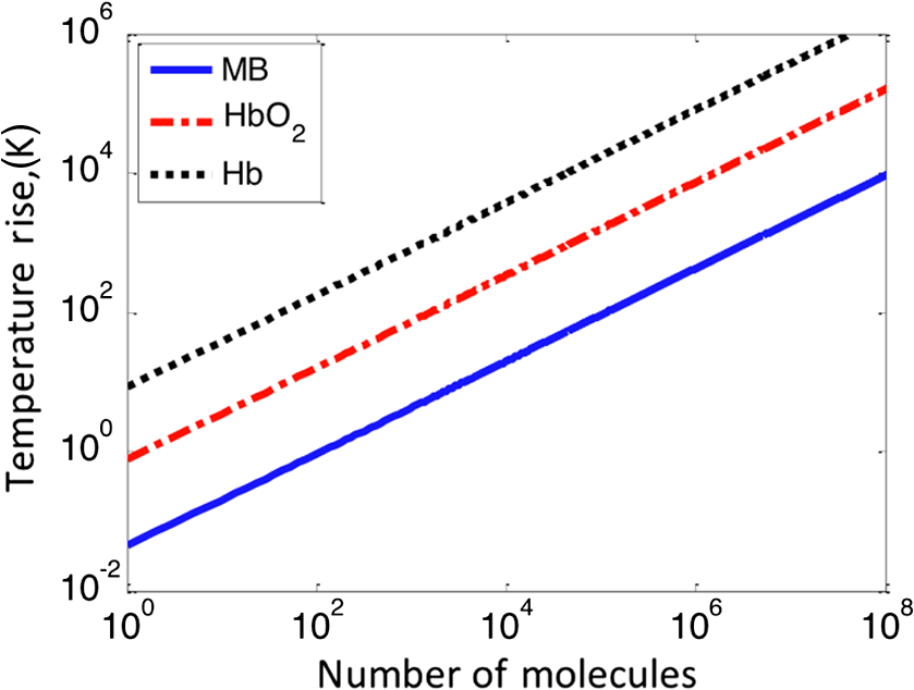
4. Experimental Results

4.1.

Sensitivity to Methylene Blue

The SNRs (as amplitude ratios) for the three concentrations of methylene blue are shown in Fig. 4 for both the pulsed-PA and CW-PA systems. The number of illuminated molecules was $3.3 \times$ greater for the pulsed-PA system than that for the CW-PA system based on calculations from Gaussian beam propagation and concentration, and the optical intensity was about $10 \times$ greater. Still, the SNRs are significantly higher for the CW-PA system than for the pulsed-PA system for all three concentrations due to the difference in bandwidth. To achieve narrowband (1.25 Hz) filtering with the CW-PA system, however, the data acquisition time was a few seconds, while the data acquisition time for the broadband pulsed-PA system was 1 ms (limited by the pulse repetition frequency of the pulsed laser). B-scan images from the pulsed-PA system showed that the standard deviation of the signal to be roughly 50% and 67% for the 0.1% and 0.01% samples, respectively. The SNR was too low for the lowest concentration sample to measure the variation. The pulsed-PA system achieved an SNR close to 1 for $1.5 \times 10^{8} \pm 1.0 \times 10^{8}$ molecules, so $NEM \approx 1.5 \times 10^{8} \pm 1.0 \times 10^{8}$ in a 50 MHz bandwidth. The bandwidth for pulsed-PA is necessarily high since the signal is broadband.

Fig. 4

Sensitivity to methylene blue for both CW-PA and pulsed-PA systems operating at two different intensity values (i.e., 3.4% and 41% of $I_{sat}$ ). The SNR is based on the amplitude ratio.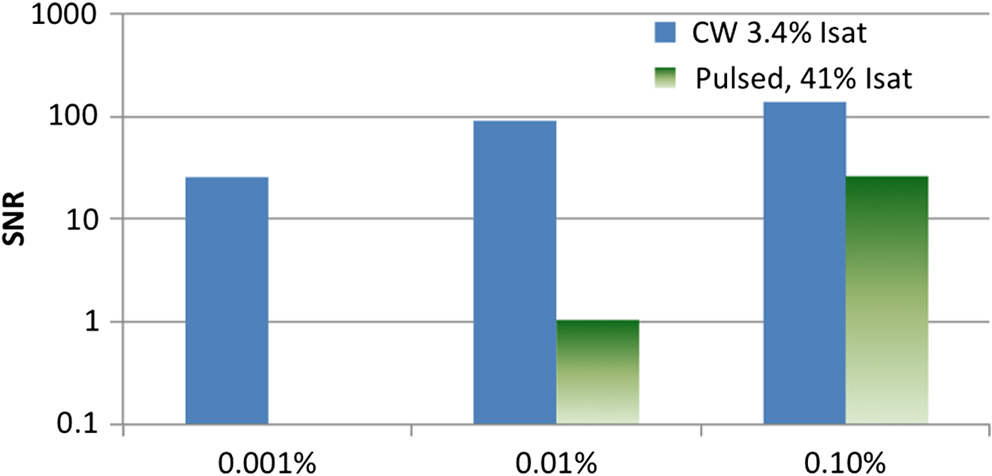

The SNR from the CW-PA system is not a linear function of concentration. We observed that the CW-PA signal from the highest concentration sample decreased significantly during the measurement window while the lower two concentration samples exhibited fairly stable signals. Since photobleaching would affect all the concentrations equally and thermal nonlinearity would enhance the signal from the higher concentration sample, thermal damage was the most likely cause of the nonlinear change in SNR with a concentration. In thermal confinement, the temperature rise, $T$ , of the illuminated volume is given by: $T = C_{n} σ I_{0} τ_{laser} / (ρ C_{p})$ , where $C_{n}$ is the concentration given as a number of molecules per volume, $σ$ is the absorption cross section, equal to $1.4 \times 10^{- 17} {cm}^{2}$ for methylene blue at 532 nm, $τ_{laser}$ is the pulse or tone burst duration (assuming it is less than the thermal confinement time), $ρ$ is the mass density, and $C_{p}$ is the specific heat. Using the beam waist, 1.4 μm, as the characteristic length, the thermal confinement time is 15 μs in water, so the 1.2 μs tone burst duration, $τ_{laser}$ , is within a thermal confinement. In fact, the thermal confinement time is slightly longer than the repetition period, 12 μs, so two tone bursts may be deposited before the heat sufficiently diffuses out of the focal zone. The focal zone, with a peak intensity of $6.5 MW / {cm}^{2}$ , experiences the highest temperatures. The temperature rise at focus, considering heat deposition from two tone bursts, is $> 100 K$ for the highest concentration sample, enough to cause damage, and 10 and 1 K for the lower two concentration samples. The average temperature rise throughout the illuminated sample volume is 4 and 0.4 K for the lower two concentration samples, so thermal nonlinearity is not expected to influence the measurements significantly. Measurements were taken at four intensity values to test this claim and demonstrated significant linearity with $R^{2} > 0.9$ (data not shown).

The SNRs for the two lower concentration samples are 92 and 25 in a 1.25 Hz bandwidth, corresponding to $NEM \approx 490,000 \pm 330,000$ and $180,000 \pm 120,000$ , respectively, using the measured 67% variation in number of molecules at 0.01%. The sensitivity is approximately 2 orders of magnitude better than the pulsed-PA system. The difference in sensitivity is anticipated due to the difference in signal bandwidth, which is roughly 8 orders lower for the CW-PA system. Since the sensitivity improves as $Δ f$ decreases, the CW-PA sensitivity should be improved by roughly 4 orders of magnitude. The limited improvement (2 orders of magnitude instead of 4) can be understood by the difference in optical intensity between the two systems, which is about $10 \times$ , and the 10% duty cycle of the CW-PA system. In theory, comparable system performance can be achieved using a pulsed-PA system by averaging $10^{8}$ pulses. The data acquisition time for $10^{8}$ pulses at the 1 kHz repetition rate used here would be 10,000 s, or 10,000 times the data acquisition time of the CW-PA system. The CW-PA system has a 1.25 Hz bandwidth so $NEM / \sqrt{Δ f} \approx 160,000 {Hz}^{- 1 / 2}$ , which is roughly 2 orders of magnitude different from the optimum values predicted in Table 1, owing to the suboptimal intensity ( $0.04 \times I_{sat}$ instead of $2.4 \times I_{sat}$ ) and duty cycle (10% instead of 100%).

4.2.

Sensitivity to Hemoglobin

Hemoglobin is the most common target in photoacoustic imaging. To measure the molecular sensitivity, the SNR was measured for four intensity values on the CW-PA system, as shown in Fig. 5. The intensity values are given as a fraction of the saturation intensity of oxygenated hemoglobin at 532 nm, which is approximately $100 MW / {cm}^{2}$ . The SNR is linear with intensity with an $R^{2}$ value of 0.999, allowing linear extrapolation to the NEM. The SNR at the highest intensity is 440 (amplitude ratio), and the number of illuminated hemoglobin molecules is $3.8 \times 10^{7}$ , indicating $NEM \approx 86,000$ for this intensity value. The signal bandwidth is 1.25 Hz so $NEM / \sqrt{Δ f} \approx 77,000 {Hz}^{- 1 / 2}$ , which is roughly 2 orders of magnitude greater than the optimum value predicted in Table 1, again owing to the suboptimal intensity ( $0.028 \times I_{sat}$ instead of $2.4 \times I_{sat}$ ) and duty cycle (10% instead of 100%).

Fig. 5

Sensitivity to hemoglobin. The amplitude signal-to-noise ratio (SNR) is shown as a function of light intensity for a 1.25 Hz bandwidth. The high $R^{2}$ value shows that the system is well approximated by a linear model.

4.3.

Imaging Hemoglobin

CW-PA imaging of the RBC sample verified the proper focal alignment and the RBC monolayer, shown in Fig. 6. For imaging, the duty cycle was increased to 100% and the image exhibited negligible electromagnetic coupling. The SNR in the image taken with a 781 Hz bandwidth was 67 (amplitude ratio). In a linear regime, $NEM / \sqrt{Δ f}$ would be around $20,000 {Hz}^{- 1 / 2}$ , which is about 4× better than previously estimated. The increase in duty cycle is expected to improve the sensitivity $10 \times$ while the decrease in intensity is expected to worsen the sensitivity $4 \times$ , so overall the sensitivity is expected to be roughly $2.5 \times$ better in a linear regime. However, since imaging was performed over a limited intensity range, the system linearity was not confirmed and thermal nonlinearity may have enhanced the signal.

Fig. 6

Imaging RBCs with narrowband CW-PAs. The amplitude SNR is 67 for 0.73%, $I_{sat}$ 100% duty cycle, and 781 Hz bandwidth.

5. Projection to Single Molecule

While the intensity and duty cycle were limited in the experiments to minimize thermal damage and nonlinear effects, fewer illuminated molecules would generate less heat and therefore facilitate higher intensity and duty cycle. The local steady state temperature rise due to constant heating (100% duty cycle) of a spherical volume of radius, $a$ , is given by $T_{ss} = N σ I_{0} / (8 π k_{w} a)$ , where $N$ is the number of absorbing molecules within the focal zone and $k_{w}$ is the thermal conductivity of water, equal to $5.2 mW / (cm K)$ . The temperature rise is shown in Fig. 7 for the optimum intensity, $I_{0} = 2.4 \times I_{sat}$ , as a function of the number of illuminated molecules for methylene blue (MB), oxygenated hemoglobin ( ${HbO}_{2}$ ), and deoxygenated hemoglobin (Hb) molecules at 5.2 mM concentration. (To calculate the local temperature rise of a decreasing number of molecules, the concentration is fixed and the radius of the illuminated sphere is decreased.) These three molecules are used to show the increase in temperature for three different lifetimes—380 ps for MB, 22 ps for ${HbO}_{2}$ , and 2 ps for Hb. The temperature rise for a single molecule is $< 0.05 K$ for MB, 0.8 K for ${HbO}_{2}$ , and 8.5 K for Hb. For MB and ${HbO}_{2}$ , the temperature rise is too small to cause either damage or thermal nonlinearity. For Hb, the temperature rise is still too small to cause thermal damage in vitro, although thermal nonlinearity may boost the signal slightly. Extrapolating from the measured data, increasing intensity from $0.034 \times I_{sat}$ to $2.4 \times I_{sat}$ for MB increases the generated pressure amplitude by $11 \times$ . Furthermore, increasing the duty cycle from 10% to 100% increases the detected signal at the lock-in amplifier by $10 \times$ , resulting in a final $NEM / \sqrt{Δ f} \approx 1500 {Hz}^{- 1 / 2}$ . The measurements of ${HbO}_{2}$ exhibit $NEM / \sqrt{Δ f} \approx 77,000 {Hz}^{- 1 / 2}$ . Increasing the intensity from $0.028 \times I_{sat}$ to $2.4 \times I_{sat}$ increases the generated pressure amplitude by $13 \times$ ; considering the $10 \times$ improvement from the duty cycle, the final resulting sensitivity, $NEM / \sqrt{Δ f} \approx 590 {Hz}^{- 1 / 2}$ .

Fig. 7

Temperature rise with number of illuminated molecules at $2.4 \times I_{sat}$ .

The molecular sensitivity is always molecule dependent. We see from Eq. (10) that molecules with shorter lifetimes can generate higher pressure amplitudes. Since de-oxygenated hemoglobin exhibits a lifetime roughly $10 \times$ smaller than that from oxygenated hemoglobin,¹⁹ the NEM may be improved to $10 \times$ .

6. Discussion

The fundamental limit of acoustic detection is thermal noise. Acoustic black body radiation, which gives rise to thermal noise, is significant at room temperature, with power spectral density around $k_{B} T \sim 10^{- 20} W / Hz$ . (For resonant transducers, this energy corresponds to tens of microPascals per root Hertz.) Chilling the medium is usually counterproductive because the efficiency of photoacoustic generation typically decreases with temperature. In order to reach single molecule sensitivity, therefore, a photoacoustic transient with power spectral density $\sim 10^{- 20} W / Hz$ must be generated. Increasing the integration time is one way to increase the photoacoustic energy. For example, with modulated CW illumination and a lock-in amplifier, the photoacoustic signal can be continuously averaged. At integration times beyond a few seconds, i.e., bandwidths $< 1 Hz$ , flicker noise (also called $1 / f$ noise or pink noise) becomes significant. For an integration time of 1 s, the photoacoustic power must be $> 10^{- 20} W$ to be detectable. The available parameters to maximize photoacoustic generation are optical intensity and frequency, which both have practical limits. The optimum optical intensity depends upon the saturation intensity of the molecule, which increases with decreasing lifetime. The optimized photoacoustic power generated from a single molecule of oxygenated hemoglobin or methylene blue before losses is computed in this work for various modulation frequencies and listed in Table 1 as $S_{g}$ . A single molecule of ${HbO}_{2}$ generates the required power, $> 10^{- 20} W$ , at frequencies beyond 125 MHz; however, acoustic attenuation and detector losses are significant in this frequency regime. An acoustic microscope lens with a radius of curvature of tens of micrometers can facilitate shorter working distances in water and further decrease losses due to acoustic attenuation. Resonant transducers with $- 6 dB$ losses are also possible in this frequency range although difficult to find commercially. Micro-resonator (optical) detection is another potential solution. The efficiency of detection increases with Q-factor and detector noise is overcome with increased optical intensity. Also, the optical detection system can probe an area small in comparison to the acoustic wavelength and therefore does not require acoustic focusing, making detection at short depths readily feasible.

We verify our theoretical estimates using a CW-PA detection system with a readily available piezoelectric transducer. With this detector, we conclude that the NEM is on the order of 10s to 1000s of molecules, depending on the lifetime of the molecule. The theory predicts the possibility of detecting a single molecule with a picosecond lifetime through detector optimization.

Acknowledgments

This work was sponsored in part by the National Institutes of Health Grant Nos. DP1 EB016986 (NIH Director’s Pioneer Award), R01 EB008085, U54 CA136398, R01 CA157277, and R01 CA159959. Lihong V. Wang has a financial interest in Microphotoacoustics, Inc. and Endra, Inc., which, however, did not support this work. Konstantin Maslov has a financial interest in Microphotoacoustics, Inc., which did not support this work.

References

1.

L. V. WangS. Hu, “Photoacoustic tomography: in vivo imaging from organelles to organs,” Science, 335 (6075), 1458 –1462 (2012). http://dx.doi.org/10.1126/science.1216210 SCIEAS 0036-8075 Google Scholar

2.

S. A. Ermilovet al., “Laser optoacoustic imaging system for detection of breast cancer,” J. Biomed. Opt., 14 (2), 024007 (2009). http://dx.doi.org/10.1117/1.3086616 JBOPFO 1083-3668 Google Scholar

3.

H. Keet al., “Performance characterization of an integrated ultrasound, photoacoustic, and thermoacoustic imaging system,” J. Biomed. Opt., 17 (5), 056010 (2012). http://dx.doi.org/10.1117/1.JBO.17.5.056010 JBOPFO 1083-3668 Google Scholar

4.

D.-K. Yaoet al., “In vivo label-free photoacoustic microscopy of cell nuclei by excitation of DNA and RNA,” Opt. Lett., 35 (24), 4139 –4141 (2010). http://dx.doi.org/10.1364/OL.35.004139 OPLEDP 0146-9592 Google Scholar

5.

C. ZhangK. MaslovL. V. Wang, “Subwavelength-resolution label-free photoacoustic microscopy of optical absorption in vivo,” Opt. Lett., 35 (19), 3195 –3197 (2010). http://dx.doi.org/10.1364/OL.35.003195 OPLEDP 0146-9592 Google Scholar

6.

L. V. Wang, “Tutorial on photoacoustic microscopy and computed tomography,” IEEE J. Sel. Topics Quant. Electron., 14 (1), 171 –179 (2008). http://dx.doi.org/10.1109/JSTQE.2007.913398 IJSQEN 1077-260X Google Scholar

7.

J. Yaoet al., “Label-free oxygen-metabolic photoacoustic microscopy in vivo,” J. Biomed. Opt., 16 (7), 076003 (2011). http://dx.doi.org/10.1117/1.3594786 JBOPFO 1083-3668 Google Scholar

8.

C. Yehet al., “Photoacoustic microscopy of blood pulse wave,” J. Biomed. Opt., 17 (7), 070504 (2012). http://dx.doi.org/10.1117/1.JBO.17.7.070504 JBOPFO 1083-3668 Google Scholar

9.

V. P. Zharov, “Ultrasharp nonlinear photothermal and photoacoustic resonances and holes beyond the spectral limit,” Nat. Photonics, 5 (2), 110 –116 (2011). http://dx.doi.org/10.1038/nphoton.2010.280 1749-4885 Google Scholar

10.

A. Danielliet al., “Non-linear photoacoustic microscopy with optical sectioning,” in SPIE Photonics West, Conference on Biomedical Optics, (2013). Google Scholar

11.

A. Gaiduket al., “Room-temperature detection of a single molecule’s absorption by photothermal contrast,” Science, 330 (6002), 353 –356 (2010). http://dx.doi.org/10.1126/science.1195475 SCIEAS 0036-8075 Google Scholar

12.

W. Minet al., “Imaging chromophores with undetectable fluorescence by stimulated emission microscopy,” Nature, 461 1105 –1109 (2009). http://dx.doi.org/10.1038/nature08438 NATUAS 0028-0836 Google Scholar

13.

S. ChongW. MinX. S. Xie, “Ground-state depletion microscopy: detection sensitivity of single-molecule optical absorption at room temperature,” J. Phys. Chem. Lett., 1 (23), 3316 –3322 (2010). http://dx.doi.org/10.1021/jz1014289 1948-7185 Google Scholar

14.

M. Celebranoet al., “Single-molecule imaging by optical absorption,” Nat. Photonics, 5 (2), 95 –98 (2011). http://dx.doi.org/10.1038/nphoton.2010.290 1749-4885 Google Scholar

15.

A. D. Pierce, Acoustics: An Introduction to its Physical Principles and Applications, 155 McGraw-Hill, New York (1981). Google Scholar

16.

A. RosencwaigA. Gersho, “Photoacoustic effect with solids: a theoretical treatment,” Science, 190 (4214), 556 –557 (1975). http://dx.doi.org/10.1126/science.190.4214.556 SCIEAS 0036-8075 Google Scholar

17.

A. E. Siegman, Lasers, University Science Books, Sausalito, California (1986). Google Scholar

18.

I. S. GradnhteynI. M. Ryzhik, Table of Integrals Series and Products, 366 Academic Press, New York (1965). Google Scholar

19.

A. Danielliet al., “Picosecond absorption relaxation measured with nanosecond laser photoacoustics,” Appl. Phys. Lett., 97 (16), 163701 –163703 (2010). http://dx.doi.org/10.1063/1.3500820 APPLAB 0003-6951 Google Scholar

20.

R. H. Mellen, “The thermal-noise limit in the detection of underwater acoustic signals,” J. Acoust. Soc. Am., 24 (5), 478 –480 (1952). http://dx.doi.org/10.1121/1.1906924 JASMAN 0001-4966 Google Scholar

21.

T. Rhyne, “Characterizing ultrasonic transducers using radiation efficiency and reception noise figure,” IEEE Trans. Ultrason. Ferroelectr. Freq. Control, 45 (3), 559 –566 (1998). http://dx.doi.org/10.1109/58.677600 ITUCER 0885-3010 Google Scholar

22.

G. D. VendelinA. M. PavioU. L. Rohde, Microwave Circuit Design Using Linear and Nonlinear Techniques, 2nd ed.John Wiley & Sons, New York (2005). Google Scholar

23.

M. Baileyet al., “Physical mechanisms of the therapeutic effect of ultrasound (a review),” Acoust. Phys., 49 (4), 369 –388 (2003). http://dx.doi.org/10.1134/1.1591291 AOUSEK 1063-7710 Google Scholar

24.

E. Z. ZhangP. C. Beard, “A miniature all-optical photoacoustic imaging probe,” Proc. SPIE, 7899 78991F (2011). http://dx.doi.org/10.1117/12.874883 Google Scholar

25.

A. OraevskyA. Karabutov, “Ultimate sensitivity of time-resolved opto-acoustic detection,” Proc. SPIE, 3916 228 –239 (2000). http://dx.doi.org/10.1117/12.386326 PSISDG 0277-786X Google Scholar

26.

C. F. QuateA. AtalarH. Wickramasinghe, “Acoustic microscopy with mechanical scanning—a review,” Proc. IEEE, 67 (8), 1092 –2206 (1979). http://dx.doi.org/10.1109/PROC.1979.11406 IEEPAD 0018-9219 Google Scholar

27.

G. A. D. BriggsO. V. Kolosov, Acoustic Microscopy, Oxford University Press Inc., New York (2009). Google Scholar

28.

A. M. WinklerK. MaslovL. V. Wang, “Towards single molecule detection using photoacoustic microscopy,” Proc. SPIE, 8581 85811A (2013). http://dx.doi.org/10.1117/12.2004265 PSISDG 0277-786X Google Scholar

29.

B. S. Fujimotoet al., “Fluorescence and photobleaching studies of methylene blue binding to DNA,” J. Phys. Chem., 98 (26), 6633 –6643 (1994). http://dx.doi.org/10.1021/j100077a033 JPCHAX 0022-3654 Google Scholar

30.

K. MaslovL. Wang, “Photoacoustic imaging of biological tissue with intensity-modulated continuous-wave laser,” J. Biomed. Opt., 13 (2), 024006 (2008). http://dx.doi.org/10.1117/1.2904965 JBOPFO 1083-3668 Google Scholar

31.

A. PetschkeP. J. La Rivière, “Comparison of intensity-modulated continuous-wave lasers with a chirped modulation frequency to pulsed lasers for photoacoustic imaging applications,” Biomed. Opt. Express, 1 (4), 1188 –1195 (2010). http://dx.doi.org/10.1364/BOE.1.001188 BOEICL 2156-7085 Google Scholar

32.

J. Yaoet al., “Double-illumination photoacoustic microscopy,” Opt. Lett., 37 (4), 659 –661 (2012). http://dx.doi.org/10.1364/OL.37.000659 OPLEDP 0146-9592 Google Scholar

Citation Download Citation

Amy M. Winkler, Konstantin I. Maslov, and Lihong V. Wang "Noise-equivalent sensitivity of photoacoustics," Journal of Biomedical Optics 18(9), 097003 (11 September 2013). https://doi.org/10.1117/1.JBO.18.9.097003

Published: 11 September 2013

Access the abstract

JOURNAL ARTICLE
11 PAGES

DOWNLOAD PAPER SAVE TO MY LIBRARY

GET CITATION

CITATIONS

Cited by 100 scholarly publications and 1 patent.

Explore citations on Lens.org

RIGHTS & PERMISSIONS

Get copyright permission Get copyright permission on Copyright Marketplace

KEYWORDS

Molecules

Photoacoustic spectroscopy

Transducers

Acoustics

Nanoelectromechanical systems

Sensors

Signal to noise ratio

1.

Introduction

2.

Theory

2.1.

Photoacoustic Signal

Eq. (1)

Eq. (2)

Eq. (3)

Eq. (4)

Eq. (5)

Eq. (6)

Eq. (7)

Fig. 1

Eq. (8)

Eq. (9)

Eq. (10)

2.2.

Noise

Eq. (11)

Eq. (12)

Eq. (13)

Eq. (14)

Eq. (15)

Eq. (16)

Eq. (17)

Eq. (18)

Table 1

3.

Experimental Setup

3.1.

Photoacoustic System

Fig. 2

3.2.

Transducer Calibration

Eq. (19)

Eq. (20)

Fig. 3

3.3.

Samples

3.4.

Signal to Noise Measurements

3.5.

Imaging

Table 2

4.

Experimental Results

4.1.

Sensitivity to Methylene Blue

Fig. 4

4.2.

Sensitivity to Hemoglobin

Fig. 5

4.3.

Imaging Hemoglobin

Fig. 6

5.

Projection to Single Molecule

Fig. 7

6.

Discussion

Acknowledgments

References

Show All Keywords

Keywords/Phrases

Search In:

Publication Years