2.1.

Cell Cultures

All the experimental protocols were approved by the Italian Ministry of Health. Primary cultures were obtained from hippocampi of mice (C57BL6J, Charles River, Milano, Italy) at embryonic day 18 (E18). Embryos were removed and dissected under sterile conditions. Hippocampi were dissociated by enzymatic digestion in trypsin (0.125% for 20 min at 37°C). Trypsin activity was blocked by adding complete media (Neurobasal2, Gibco, Milano, Italy) supplemented by B27 (2%, Gibco, Milano, Italy), alanyl glutamine (2 mM, Gibco, Milano, Italy), and penicillin/streptomycin (both 1 mM, Sigma, Milano, Italy) containing 10% fetal bovine serum (FBS, Gibco, Milano, Italy). After trypsinization, tissues were rinsed in complete media without FBS and dissociated with a plastic pipette. Neurons were plated at a concentration of $30,000\text{cells}/\mathrm{ml}$ on glass-bottom Petri dishes (P35G-0-14-C, MaTek Corporation, Ashland), whose surface had been treated with poly-d-lysine (0.1%, Sigma, Milano, Italy) to allow cell attachment. These plated neurons were kept in the incubator for 2 h, allowing them to attach, and thereafter, the dishes were filled with 3 ml of serum-free medium. Experiments were carried out with neurons at 2 DIV.

In order to evaluate the cell viability after a long-term imaging experiment, the neurons were stained with a modified fluorescein diacetate/propidium iodine staining protocol.¹³ Cells were stained for 3 min at room temperature with $15\mu \text{g}/\mathrm{ml}$ fluorescein diacetate, $5\mu \text{g}/\mathrm{ml}$ propidium iodine, and $3.3\mu \text{g}/\mathrm{ml}$ Hoechst-33342 (Sigma, Milan, Italy) in Tyrode solution (NaCl 140 mM, KCl 4 mM, ${\mathrm{CaCl}}_2$ 2 mM, MgCl 21 mM, glucose 10 mM, and Hepes10 mM; pH 7.4). Cells were then washed in Tyrode solution and imaged by the fluorescent module of the inverted Nikon microscope (see Sec. 2.2) equipped with a CFI Plan Apo VC $20\times$ NA 0.80 air objective. The cell-permeable fluorescein diacetate dye is retained in viable cells with intact cell membrane because of ongoing esterase enzymatic activity, while the cell-impermeable propidium iodine dye can only enter dead cells with compromised cell membrane integrity. The nuclear Hoechst-33342 dye marks both viable and dead cells and is used to count the total number of cells.

For the assay, we used cultures in two different experimental conditions: the cultures in the microscope incubator chamber, in which 2 days of long-term imaging was performed, and the cultures coming from the same cell-culture preparation but retained in the bench incubator. The neuron viability of both cultures was monitored after the 2 days of long-term imaging. At the end of the staining procedure, we selected nine random fields for each sample, obtaining a total of 45 images per condition. Images were then analyzed with ImageJ software ( http://rsbweb.nih.gov/ij/) to count the total cell number and the number of live and dead cells.

2.2.

Optical Microscope

We used a commercial inverted microscope Nikon Ti-e (Nikon Instruments Europe B.V., Amsterdam, The Netherlands) equipped with DIC contrast fluorescence epi-illuminator including a mercury arc lamp HBO 103 W (OSRAM GmbH, Munich, Germany) and filter set cubes for distinct dyes [4',6-diamidino-2-phenylindole (DAPI), Fluorescein isothiocyanate (FITC), and Tetramethylrhodamine isothiocyanate (TRITC)]. The Nis-Elements (Nikon Instruments Europe B.V., Amsterdam, The Netherlands) microscope software controls the filter wheels, microscope stage, and light source. During long-term time-lapse experiments, we did not use water- or oil-immersion objectives, because it is difficult to avoid the evaporation of the immersion medium. Moreover, the microscope objective makes contact with the heated culture dish and creates a temperature gradient, which produces fluid flow, and long-term cell viability cannot be achieved. We chose the Nikon Plan Fluor $40\times$, 0.75 NA DIC air objectives, which provide a good magnification/numerical aperture ratio, and thus, good light collection efficiency. The system is equipped with a back-thinned electron-multiplied (EM)-CCD Andor Camera Ixon DU897 (Andor Technology plc, Belfast, UK).

The microscope stage is equipped with the Nikon Perfect Focus System (PFS) (Nikon Instruments Europe B.V., Amsterdam, The Netherlands), in order to eliminate axial focusing fluctuations. The unit operates in stand-alone mode without a software interface to the host computer. This device allows performing long-term time-lapse experiments eliminating the mechanical drifts and environmental noises, if there is a change in the room temperature. Moreover, the motorized stage (Nikon TI-ER, Nikon Instruments Europe B.V., Amsterdam, The Netherland) allows programmable stage-sequential scanning of distinct regions of the sample to perform multipoint long-term imaging experiments. Thus, we could improve our statistics by parallel acquisition of distinct developing neurons. The illumination sources are time gated and synchronized with the microscope stage motion to collect images and to avoid prolonged light exposure.

2.3.

Microscope-Incubator System

The micro-incubator consists of three main parts: the chamber or case isolating the sample from external environment, the heated petri-holder controlling the sample temperature (Fig. 1), and the atmosphere control system. To design this chamber, we used an Eden 250 Objet (GmbH, Rheinmünster, Germany). The three-dimensional (3-D) printing system produces 3-D solid prototype from a digital model. Indeed, fast prototype modifications to adapt the chamber to different microscopes and sample holders represent a easy and cost-effective procedure flexible to carry out further improvements on the custom design and share it with other laboratories.

Fig. 1

Micro-incubator system. (a) Exploded view of the micro-incubator system composed of three main parts: the cover (top), the heated Petri holder (center), and the box (bottom). H indicates the insert for the humidity sensor and T indicates the insert of the thermocouple monitoring the holder temperature. (b) Photos of the cover, the heated Petri holder, and the box. Gin and Gout indicate, respectively, the input and the output of the gas mix, and P indicates the connector of the heated cover glass window to the power supply. (c) Photo of the whole micro-incubator with humidity sensor mounted in H, and the gas tubing (connected to Gout) to monitor the ${\mathrm{CO}}_2$ inside the micro-incubator, and S is the humidity sensor control.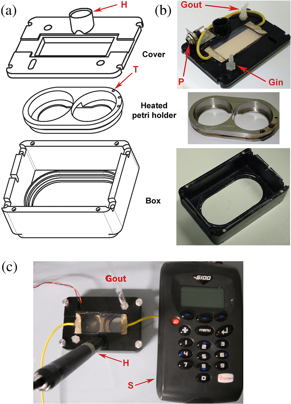

The chamber is constructed with an acrylic-based photopolymer resin (VeroBlack FullCure, Objet GmbH, Rheinmünster, Germany) which has a small thermal-inertia allowing the isolation of the microscope body from the heating part inside the micro-incubator. The chamber is made from two distinct parts: the box and the cover. The box is anchored to the microscope stage with four screws to minimize sample drifts. The bottom part of the box facilitates the housing for the heated sample holder: the border of the housing position is designed to create a shallow-collecting water condensation inside the micro-incubator, in order to avoid water seepage into the microscope objective which could cause the loss of the focus position.

Optical window is covered by a glass that is coated with a film of indium oxide acting as an electrical conductor with a resistance of about 140 Ω. Two electrical wires are connected to the glass with silver electrical conductive epoxy glue (Epoxy Technology Inc., Billerica). We apply a voltage (about 6.2 V) to the wires with a power-supply DC regulator (Life Electronics S.p.A, Riposto, Italy). The wires are oriented to have a homogeneous electrical field, and therefore, heat the glass homogeneously. We covered the glass with a film of transparent nail polish to electrically isolate it from the environment. Eight Neodyum Disc Magnets (Eclipse Magnetic Ltd., Sheffield, UK) fix the cover to the box. We need to heat the glass window to avoid the formation of water droplets (formed from water condensation) filtering or deflecting the light source, and thus, hampering the quality of bright-field imaging [see Fig. 2(b)].

Fig. 2

Long-term bright-field imaging of developing hippocampal neurons. (a) A mouse hippocampal neuron (from a cell culture at 2 DIV) with a rounded morphology at an initial stage of development, which starts to polarize [black arrow in the first frame of (a)]. During development, the extruding neurite alternates phases of growth, retraction, and branching. Bar is 10 μm. Numbers indicate minutes. (b) Background image intensity normalized to the intensity $I0$ (image background intensity of the first frame of the long-term time lapse experiment). The gray line indicates the $I/I0$ when the glass window is not heated. The black line indicates the $I/I0$ when the glass window is heated to avoid water condensation. (c) Osmolarity of the culture media measured at the end of the experimental session in 12 different experiments. The values are normalized to the osmolarity measured (in osmol/L) at the beginning of each experiment ($t=0$). (d) Percentage of cell mortality in cultures (at 5 DIVs) maintained in the bench incubator (Ctrl) and in the micro-incubator after 2 days of long-term bright-field imaging. The values of cell mortality are normalized to the average value of cell mortality for cultures at 5 DIVs maintained in the bench incubator.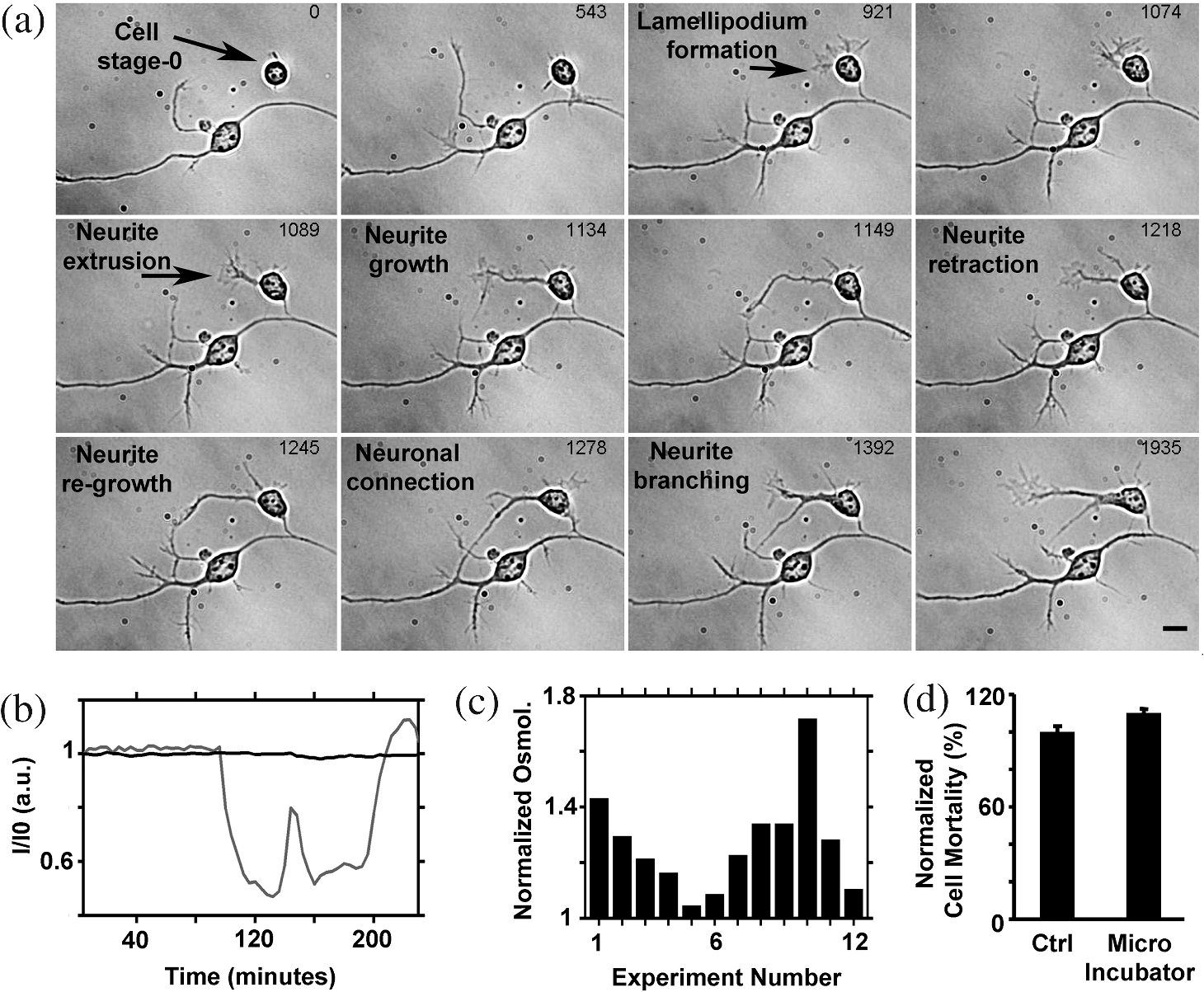

The heated Petri holder is composed of a metal body (stainless-steel holder) accommodating one or two Petri dishes inserts (for experiments requiring comparison of control and treated samples).

The round or elliptic shape of the holder is required for homogenously heating the sample without generating temperature gradient inside the Petri dish. An enameled wire (CuNi44 ø 0.253 mm, Elektrisola Dr. Gerd Schildbach GmbH&Co.KG, Reichshof-Eckenhagen, Germany) is wrapped around the holder. We chose this wire because it has high resistivity (0.49 Ω mm) minimizing the number of turns around the holder to avoid wire breaks. The wrapping wire was covered with epoxy glue to preserve the enamel and to isolate the wire from the humidity inside the micro-incubator. This kind of thermistor has been inserted in a small hole drilled in the metal body [see Fig. 1(b)]. The equivalent resistance of the wire was of 20 Ω, and we powered it by a temperature controller TC-324B (Warner instruments, Hamden, Connecticut, USA) presenting a thermistor-readout system to set a feedback control on the holder’s temperature.

To seal the bottom part of the micro-incubator, the heated Petri holder border was filled with Dow Corning high-vacuum grease (Dow Corning Europe SA, Seneffe, Belgium).

In order to maintain a narrow range of pH (between 7.2 and 7.4), it is possible to use a synthetic biological buffer such as Tris and HEPES. However, HEPES results in dramatically reduced growth rates. In addition, HEPES increases the toxicity during live-cell imaging experiments, presumably due to the increased free-radical formation coming from the synthetic buffer.¹⁴ For these reasons, we continuously flux into the micro-incubator air that composes of 5% ${\mathrm{CO}}_2$ and aqueous vapor. The gas mix was produced by a manual gas mixer (CO2BX, Okolab S.R.L, Napoli, Italy). Then, the gas mix is bubbled in a water reservoir, and it passed through an antibacterial filter unit (Midisart 2000, 0.20 μm, SartoriusAG, Goettingen, Germany) before entering the chamber. Furthermore, the atmosphere flux in generates a positive pressure inside the micro-incubator, avoiding external contaminations of the sample. To control the level of aqueous vapor in the gas mix, the reservoir is heated by an etched foil silicon heater ($10\times 10\mathrm{mm}$ with 14.4 Ω resistance, RS Components S.p.A, Milano, Italy) powered by a power-supply DC regulator (Life Electronics, S.p.A, Riposto, Italy).

Finally, evaporation of the medium results in an increase in osmolarity, which results in a consequent osmotic shock to cells in culture. To avoid this, we filled the Petri dish with neuro-basal media (about 3 ml), and we covered it with poly-dimethylsiloxane fluid (Fluid PDMS 200, density $0.913\mathrm{g}/\mathrm{ml}$, Sigma Aldrich, Milano, Italy) that is permeable to the ${\mathrm{CO}}_2$ but not to water.¹²

To continuously monitor the atmosphere inside the micro-incubator, the cover of the micro-incubator has an insert for a humidity sensor and a tube for aspiration of the internal atmosphere [see Fig. 1(c)]. The sensor and the tube are connected to a ${\mathrm{CO}}_2$ and humidity analyzer (G100, Geotech, Leamington Spa, UK) to record, and thus, recalibrate the micro-incubator atmosphere.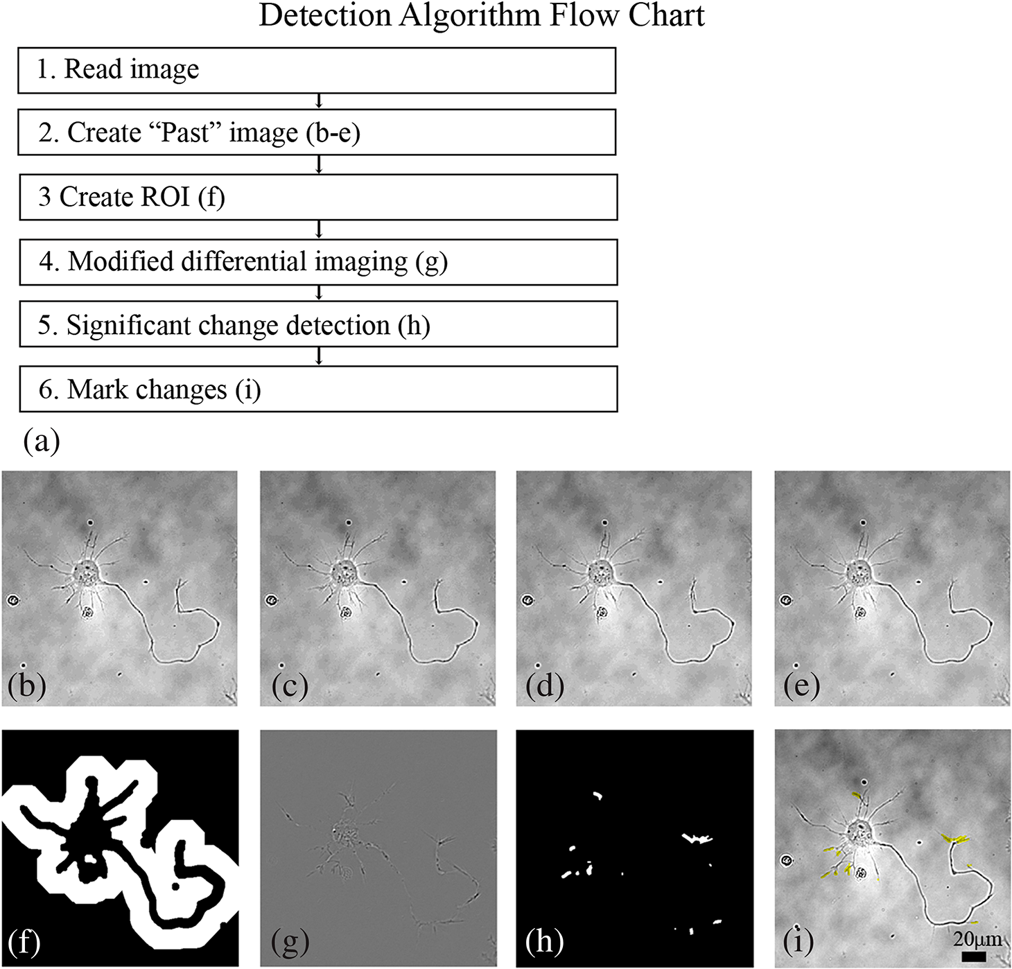

3.1.

Preprocessing

Experiment duration is usually longer than a day. During that time, the lighting conditions may change gradually in time. Since we use differential imaging over a short gap of time, the detection process is not affected by those changes.^19,20 In addition, there may be minor movement of the imaging system or object, which may cause registration differences between sequential images. To reduce registration error during imaging, we used the object stabilizer tool of the Huygens image-processing software package (Huygens, Scientific Volume Imaging, The Netherlands).

3.2.

ROI Definition

The ROI definition is performed by applying on the averaged “Past” image (see Sec. 3.3), an edge-detection operation (we chose to use “canny” algorithm, which is less likely than the others to be fooled by noise), followed by dilation operation with a disk shape (larger than the typical distance between the edges of the same object and the typical holes and gaps) and erosion with a smaller disk shape.

3.3.

Neuron Detection

The key method to detect neuron activity and growth is looking for activity around its body. The neural activity can be divided into two types: fast changes due to growth cones, spines, and lamellipodia movements, which changes from frame-to-frame (few minutes) and slow changes such as neuronal growth which takes a longer time (tens of minutes and more). Detecting the slow-changing neural image has two roles: marking the area around the neuron as ROI and acting as reference for modified differential imaging. Instead of applying simple one-step image differentiation, we compare (by subtraction) each image to a moving average (in time).

For each image at a given time step, a “past” image is produced [Figs. 3(b)–3(e)]. The “past” image is created by a set of sequenced images, which are followed by the processed image (e.g., if frame #10 is being processed, the past may be calculated from frames 1 to 9). The “past” image will be produced by averaging the image set. The goal of this operation is to reduce contrast of changes at high-time frequency and to enhance contrast of almost-constant elements. One needs to define how many images are relevant as the “past.” Of course, it depends on the frequency of slow changes such as neuron growth and the image acquisition frame rate. The “past” time window (in terms of number of frames) should be chosen in such a way that fast changes will be averaged to minimum and filtered out, while slow changes are kept and magnified. For slow frame rate, such as 2 minutes between the frames, a set of eight frames was chosen, and for higher frame rate, such as 3 seconds, five frames were sufficient. This parameter is chosen once for each set of image stacks.

3.4.

ROI-Based Image Processing

Using the “past image,” in which the constant slow-changing elements are enhanced, we apply the ROI definition processing previously defined (at Sec. 3.2). The output of this operation is a bitmap map of the neurite area and dirt. We remove dirt by keeping only the largest segment, so we have the neurite shape map. Next, we use a large dilation operation, using a disk shape larger than the typical size of the spines and cones, to “blow” the neuron shape. We then subtract the neuron shape itself, so the output is a bitmap image of the area around the neuron, defined as a significant change ROI [see Fig. 3(f)].

3.5.

Differential Imaging

The inspected images are in low contrast and with a nonuniform background (due to nonuniform lighting condition and content). The information we wish to extract lies only in the temporal changes. To enhance the temporal change a differential-imaging algorithm is used, where each image is compared with the previous one by subtraction operation. However, in our case, simple time-differential operation is not sufficient. Since the growth cones and spines appear at every image and with high frequency in time, we found it more reliable to compare each image with a moving average of a small time window of its recent past, which is actually the image we called “past” and represents the neural semi-constant shape. In this way, each frame is not affected by the growth cones and spines of the previous ones.

Each image, referred as “now,” is compared with its “past image” [see Fig. 3(g)].

3.6.

Significant Change Detection

The modified differential-imaging operation is followed by edge detection, which consideres only those within the ROI.

4.1.

Long-Term Live Imaging and Cell Motility Detection

A variety of commercial microscope chambers to perform live imaging is already available. They fall into two categories: open and closed chambers. An open-chamber system allows quick access to the cell culture but requires larger microscope enclosures to maintain the temperature and the physiological percentage of ${\mathrm{CO}}_2$ and humidity in the atmosphere around the cell culture. Such enclosure can offer superior temperature stability (as the entire microscope is heated) but requires a long time to stabilize ($>12\mathrm{h}$), which can be cumbersome; it requires expensive modifications for upgrading and does not ensure sterility of the sample. In contrast, a closed-chamber provides better insulation from the external environment and does not require complex microscope adaptation. Therefore, we developed a micro-incubator system in closed-chamber configuration (see Fig. 1). The micro-incubator characteristics are: small dimensions ($9.5\times 6.5\times 2.5\mathrm{cm}$), lightweight ($<200\mathrm{g}$) that allows an easy adaptation to any optical microscope, in situ monitoring (not provided in commercial system) of ${\mathrm{CO}}_2$, and humidity of the internal micro-environment (see Sec. 2 and Fig. 1) The possibility to calibrate the micro-incubator system by local monitoring of the atmospheric parameters is crucial because of its small dimensions, and it results necessary for long-term live-imaging experiments. Indeed, small changes in the output of gas-mixer devices could produce significant deviation from the physiological parameters of the cell cultures. With the developed micro-incubator device, we were able to perform routinely long-term bright-field imaging on a time window of 2 days [or longer, see Fig. 4(d)] and with a time resolution of one frame every 2 min. The main limiting factor is phototoxicity, and increasing time resolution, the time window in which cells remain viable decreased. Moreover, it is not possible to follow more than 10 neurons per Petri dish (with a double Petri holder, we acquired a maximum of 20 neurons per experiments) to avoid too frequent cyclic light exposure of cell culture inducing considerable phototoxicity (see Sec. 2.2). To ensure a reasonable image quality, in order to apply the image processing, we added a heated glass window. Without heating, the illumination condition of the sample was modified by water condensation on the glass surface already after 1 h [see Fig. 2(b)], that provoked significant fluctuations of the light intensity hampering the image quality. With our micro-incubator, we reached a stable $5\%\pm 0.2\%$ ${\mathrm{CO}}_2$ and 90% humidity content in the internal environment and a small evaporation of the medium in the Petri dish (0.3 ml in 40 h of long-term imaging). Medium evaporation increases the osmolarity, which in turn induces osmotic shock causing cell swelling and subsequent shrinking [see Fig. 4(a)]. In Fig. 2(c), we report the increase in osmolarity measured after $\sim 40\mathrm{h}$ of long-term imaging in 12 distinct experimental sessions. The starting osmolarity was $220\pm 10\mathrm{osmol}/\mathrm{ml}$ and with an increase of about 30% in 40 h, no-significant cell osmotic shock was detected. Figure 2(d) shows that cultures in the micro-incubator system present a slight increase of cell mortality (about 10%) when compared with cultures maintained in the incubator, which indicates the suitability of the developed closed-chamber system.

Fig. 4

Examples of long-term bright-imaging failures and successes. (a) Cell suffered osmotic shock and shrank, due to a fast osmolarity increase in the culture media. (b) Cells died due to bacterial contamination (see bacteria in the last frame). (c) Long-term imaging with no Perfect Focus System (PFS) (see Sec. 2). The focus position was lost, and the long-term live imaging session was compromised. (d) Long-term imaging of mouse hippocampal neurons starting at 2 DIV and lasting for about 4 days. Bars are 10 μm. Numbers indicate time in hours:minutes.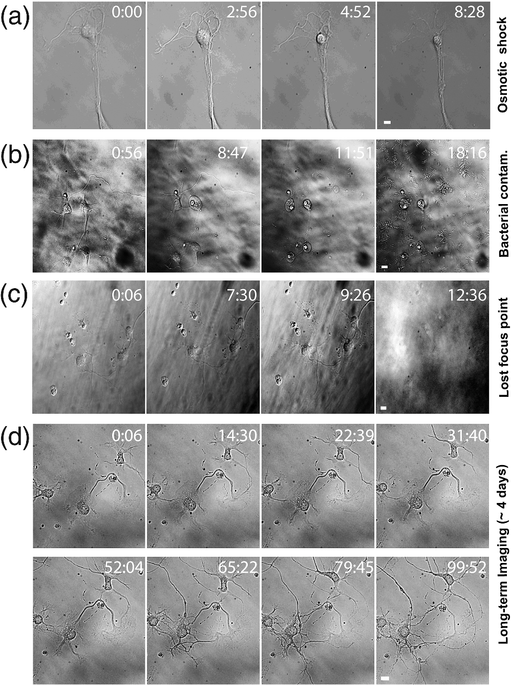

With the above-mentioned calibration parameters of the micro-incubator, we were able to follow neuronal development in cell cultures starting from 2 DIVs. In Fig. 2(a), we illustrate an example of a cell with round shape that is starting to polarize. Evident is the formation of a small contact with the neighboring cell after 9 h and the formation of a lamellipodium around the cell soma after around 15 h. During membrane ruffling, a cellular protrusion extrudes from the lamellipodium after about 18 h [1089 minutes in Fig. 2(a)]. Such cell protrusion presents a complex dynamic composed of growth and retraction phases, formation of a neuronal connection with another cell, change of the neuronal connection position, and neurite branching with formation of another protrusion.

Although DIC imaging provides a better contrast of thin and transparent samples, it requires higher light intensity through the sample, which leads to higher phototoxicity. Therefore, we performed bright-field imaging with the aim to provide a stable signal-to-noise ratio that allows the use of fixed algorithm parameters for image analysis. The example illustrated in Fig. 3 shows the strength of the proposed algorithm (see Secs. 2 and 3); also with a low-contrast image sequence, the algorithm is able to detect small changes (indicated in yellow) of the neuronal morphology.

In Fig. 5, we illustrate an application of the hardware-software system: the detection and the quantification of neuronal motility during growth. In Fig. 5(a), the algorithm was able to detect the formation of a growth cone-like structure (actin wave) along the axon of a developing neuron. Moreover, the algorithm detects the changes in the shape of the actin wave and its motility flow along the major neurite. Actin waves form along neurites with a frequency ranging from 0.2 to $1.5\text{wave}/\mathrm{h}$⁸ and move along neurites with an average velocity of $2.2\mu \text{m}/\min$.¹² With the provided temporal resolution of one frame for every 2 min, we are oversampling actin-wave formation with a factor of more than 30, and we follow their movement along the neurite with a precision of 400 nm (pixel dimension) for every 2 min (time resolution). In Fig. 5(b), we show the tracking of a growth cone. The proposed detection algorithm is able to detect changes in the morphology of the growth cone during neurite growth.

Fig. 5

Detection of cell motility flow. (a) Detection of an actin wave formation, and its propagation toward the tip of the neurite. (b) Detection of growth-cone motility and neurite growth. Yellow areas indicate the algorithm-detected significant changes in the field-of-view. Bar is 10 μm. Numbers indicate minutes. (Video 1, MOV, 293 KB) [URL: http://dx.doi.org/10.1117/1.JBO.18.11.111415.1].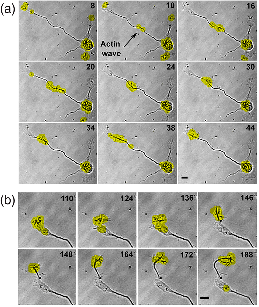

4.2.

Actin Waves and Dynamics at the Neurite Tips

The stack of change masks indicated by yellow marks in the images [stack of binary images containing only the data from the yellow marks: image example in Fig. 3(h)] is used to measure and quantify cell motility. For example, it allows measuring and quantifying actin waves’ velocity and frequency along the major neurite [see Fig. 6(a)]. As a first step, a single image is used to detect the neurite shape as a curved line. Such curved line represents the reference axes to define the location of the yellow marks on the neurite starting from the soma ($\mathrm{soma}=0$) and ending at the tip [$Y$-axis of graph in Fig. 6(b)]. Only yellow marks that are located at less than 16 μm from the neurite edge are counted. The center of mass of each yellow mark is projected on the neurite axes. In such a way, on the graph in Fig. 6(b), the position along the neurite of all the detected yellow marks over time is reported to visualize the overall motility. The size of the dots representing the detected morphology change is proportional to the area of the corresponding yellow marks. From such a plot, it is evident that the major activity is concentrated at the base and at the tip of the neurite, and a less dense cloud of points is present in the central region of the neurite. In two cases, the clouds of points in the central region become dense, and they show a linear trend toward the tip. The cloud of points represents an acting wave travelling to the neurite tip. Thus, with the proposed detection algorithm, it is possible to measure the velocity of the actin waves by a linear fit of the cloud of points. In the cell shown in Fig. 6(a), we detected two actin waves, and we measured a velocity of $2.9\pm 0.2\mu \text{m}/\min$ (first wave) and $3.2\pm 0.1\mu \text{m}/\min$ (second wave), which appears with a time gap of $39\pm 5\min$ [graph in Fig. 6(b)]. The wave velocity was calculated by applying a weighted least mean square linear fit to the related cloud of points with yellow marks area as weight.

Fig. 6

Actin waves and dynamics at the neurite tips. (a) Bright-field image of a hippocamapal neuron (2 DIVs). The image shows the detection of activity (yellow marks) along the neurite and the coordinates of their localization (L) and size (A) (starting from the soma and ending at the tip of the neurite). (b) Plot of cell dynamics along the neurite. “Yellow marks,” which are the significant changes of detected cell morphology, are used to quantify tip activity and neurite flow (actin waves) at a maximum distance of 16 μm from the neurite in time ($\text{location on the neurite}=Y\text{-}\text{axis}$). The size of the dots is proportional to the area of the yellow marks. Actin waves appear as cloud of points fitted with a linear trend lines (magenta color), where the slope of the line is equal to the wave velocity. Two waves have been significantly detected with velocity of $2.9\pm 0.2\mu \text{m}/\min$ (first wave) and $3.2\pm 0.1\mu \text{m}/\min$ (second wave), which appears with time gap of $39\pm 5\min$. Linear trend line was calculated by least-mean square liner fit with yellow mark area as weights. Vertical magenta lines indicate the arrival of the actin waves to the tip. (c) Tip of the major neurite of the neuron in (a) with superimposed polar coordinates used to quantify the tip motility. The tip position is (0, 0), and the angles are measured in the clockwise direction, starting from the line oriented along the distal part of the major neurite. (d) Plot of angular coordinates of the yellow marks detected around the tip. (f) Plot of the distance between the detected yellow marks and the position of the neurite tip. In (d) and (f), the areas of branching of the tip motility are labeled in light blue and light red. (e) Color-coded map of the dynamic of the neurite tip, calculated as the number of the folds in which a yellow mark was detected in each pixel of the image. The higher amount of activity is in red, the lower in dark blue.

To quantify the growth-cone dynamics at the tip of the neurite, we measured the position of the yellow marks in polar coordinates [Figs. 6(d) and 6(f)]. We defined the center of the polar coordinate at the location of the growth cone in the first frame and the origin of the angular coordinate by a line parallel to the direction of the distal part of the neurite [see Fig. 6(c)]. Hence, we could quantitatively represent the exploratory motion of the growth cone, and therefore, the growth of the neurite itself. Also in this case, the dot size is proportional to the detected yellow mark area. Starting from the first frame, we observed random-like activity at a wide-angle range and at short distance from tip [graphs in Figs. 6(d) and 6(f)]. After the first wave reached the tip [marked with a vertical magenta line in the graph of Fig. 6(b)], the activity changed to a narrow angle with larger yellow mark area size. After the arrival of the second wave, the tip search activity (marked with a second vertical magenta line) changed again. At this point, the growth cone moved with two angles at two slightly distinct distances, and the distance of the yellow marks from the origin of the polar coordinate increase faster. Later on, the movement of the tip occurred at two well-distinguished angles and at two different distances [marked in light blue and light red in Figs. 6(d) and 6(f)]. In Fig. 6(e), the spatial activity of the growth cone is represented by a color-code map obtained by the sum of the number of times a change of morphology was detected for each pixel of the frame.

4.3.

Dynamics at the Cell Body

During neuronal polarization, in parallel with the elongation of a longer neurite which will become the axon, other neurites, the dendrites, start to growth from the soma, and they will functionally connect to other neurons. In order to understand if their growth is correlated in time, we quantified the cell motility around the soma. A circular area, with a radius of 60 μm, was marked around the soma and divided into eight sectors [starting from right side, CCW as shown in Fig. 7(a)]. The measure of the motion activity in each sector was given by the number of yellow pixels in time [Fig. 7(b)]. In order to group the sectors with similar activity, we applied principle component analysis (PCA) either on the temporal fluctuation [Fig. 7(c)] or on the spectrogram fluctuation of sector activities reported in Fig. 7(d). From this quantitative analysis, it appears that sectors 6 and 7 have different activity (both in time and frequency) in respect to the others. Moreover, while all the other sectors belong to the same group in the time PCA, it is worth noting that in the spectrogram-PCA, some sectors presented paired similarity: sectors 1 and 4, sectors 2 and 3, with sectors 5 and 8 in between these two groups. Such results indicate that, although all neurites around the soma are more or less growing simultaneously, their way of oscillating near the soma could be different in terms of frequency, and it could represent the stage of elongation of the neurite itself. In sector 8, which contains the longest neurite, most of the activity is not visible since it is localized at the tip of the neurite, outside the 60 μm radius of the circle in Fig. 7(a). Consistently, sectors 6 and 7, where movement is distinct in respect to other sectors, contain short neurite presenting or only a lamellipodia with not-yet defined cell protrusions. Further experiments and data analysis with the proposed system will allow the investigation of how the motility around the soma and the transport of material from cell body to the tip of the neurites change during its elongation phases.

Fig. 7

Dynamics at the cell body. (a) A circled area around the soma, with radius of 60 μm, is divided into eight sectors (starting from right side, CCW). Each sector activity is measured as the number of yellow pixels in time. (b) Spectrograms of the activity around the soma, for each sector, in 1000 min. A principle component analysis (PCA) method is used in order to group the sectors, both by temporal data (c) and by spectrogram (d).