1.1.

Molecular Imaging

Molecular imaging refers to a class of biomedical imaging techniques that noninvasively image biochemical differences within a living organism.¹ Molecular imaging modalities often make use of contrast agents that specifically target a particular biochemical difference, and these contrast agents are detected with systems that exploit high-sensitivity detection principles. As examples, both positron emission tomography and single photon emission computed tomography rely on the detection of individual gamma rays; fluorescence-based molecular imaging relies on cooled CCD technology capable of detecting single photons. Unfortunately, the high sensitivity of these imaging techniques comes at the expense of low spatial resolution.^1–4 In comparison, there exist biomedical imaging techniques, such as magnetic resonance imaging, ultrasound, and x-ray computed tomography, which can be classified as “anatomical” because these techniques have high spatial resolution, but lack the high sensitivity of molecular imaging and thus are more suited to high-resolution anatomical (rather than functional) images.

Nanodiamond imaging, previously introduced by us in Ref. 5, is an example of a molecular imaging technique because it relies on an imaging agent—biologically tagged nanodiamonds containing the negatively charged nitrogen-vacancy (NV) color center^6–8—to specifically highlight biochemical differences of interest. The positions of the nanodiamonds can be determined noninvasively via optically detected electron spin resonance of the NVs. Perhaps the most distinguishing feature of nanodiamond imaging relative to other molecular imaging modalities is that by combining the high sensitivity of optical detection and the high spatial resolution of magnetic resonance in a magnetic field gradient, nanodiamond imaging could potentially achieve an imaging sensitivity comparable to molecular imaging techniques but at a spatial resolution comparable to the anatomical techniques.

In our previous work, we showed how nanodiamond imaging with reasonable sensitivity improvements would be able to detect a mass of imaging agent as low as 100 fg (and perhaps as low as 25 ag), a sensitivity similar to existing molecular imaging techniques. The spatial resolution of nanodiamond imaging is limited only by the strength of the magnetic gradient and strain in the nanodiamonds, but it could easily approach 100 μm. Previously, we provided the first demonstration of imaging by optically detected magnetic resonance (ODMR) within scattering tissue, and we demonstrated two-dimensional (2-D) imaging over a $1\times 1\mathrm{cm}$ field of view up to a depth of 12 mm in chicken breast. In this paper, we review the operating principle of nanodiamond imaging, and we detail a new system that was built with a field of view ($30\times 200\mathrm{mm}$) large enough to image a mouse. We image phantoms that demonstrate the increased field of view and that are imaged with higher contrast than by the first system because of the choice of microwave frequency (2.872 versus 2.869 GHz). We explain how the choice of microwave frequency affects the imaging point-spread function by deriving a model of the ODMR lineshape of NVs in nanodiamond powder that starts with the NV spin Hamiltonian.

1.2.

Nitrogen-Vacancies in Nanodiamond

Nanodiamonds are an ideal substrate material for nanoparticle-based contrast agents. They are nontoxic and can be synthesized through scalable fabrication methods, and the biological properties of the nanodiamonds can be tailored (for example, to seek out tumors) by the facile conjugation of biological molecules to their surfaces.^9–13 With the inclusion of NVs in the nanodiamonds, they become stable, bright fluorescent probes (fluorescent nanodiamonds or FNDs) that are an alternative to bleachable organic dyes and toxic quantum dots for biological experiments.^14,15 However, it is the NVs’ spin-dependent fluorescence that enables superior spatial resolution compared to fluorescence-based molecular imaging.

The negatively charged NV is a paramagnetic diamond defect ($S=1$) formed by an adjacent nitrogen atom and lattice vacancy along the $\langle 111\rangle$ axis. While diamond’s large bandgap allows optical excitation and NV fluorescence to easily pass through it, it also causes the NV to act like an isolated atom as the electronic orbitals are tightly confined to the defect center. The presence of an “isolated atom” in a solid-state system implies that quantum effects should be visible without the ultracold temperatures and ultrahigh vacuums of atomic physics experiments. Indeed, it is possible to observe the spin state of a single NV, even at room temperature.¹⁶ This is due to the NV’s excellent quantum properties; even in nanodiamond, an NV might have a spin relaxation ($T_1$) time of $\sim 1\mathrm{ms}$ and a spin coherence time ($T_2$) of $\sim 1\mu \text{s}$.¹⁷ The key features of the center that we exploit are optically induced spin polarization and optical spin readout.

Although we describe our imaging technique in terms of nanodiamonds containing NVs, the concept extends to any combination of nanoparticle host and paramagnetic defect such that the defect can be spin-polarized optically and its spin state read out optically. Ideally, the defect spin has a reasonably long $T_1$ and $T_2$ time—longer $T_1$ allows greater spin polarization with the same optical excitation intensity (improving the imaging system’s sensitivity), and longer $T_2$ improves spatial resolution. The excitation and fluorescence should be efficient and in the near-infrared window in tissue¹⁸ for greatest optical penetration, and spin transitions should occur at frequencies where the microwave energy penetrates significantly deeper than the optical energy such that microwave penetration is not the limiting factor.

In Fig. 1(a) we see a schematic overview of the NV electronic-level structure. The ground state is a spin triplet, ${{}^3\mathrm{A}}_2$, with sublevel $m_s=0$ lying below sublevels $m_s=\pm 1$ by 2.869 GHz, as shown in Fig. 1(b). Microwaves resonant with the $0\to +1$ and $0\to -1$ transitions of the ground state transfer the NV between those spin sublevels. In the presence of a magnetic field [right side of Fig. 1(b)], the $m_s=\pm 1$ levels split relative to each other at a rate of ${56\mathrm{GHz}\mathrm{T}}^{-1}$, due to magnetic dipole interaction of the NV spin with the magnetic field; this is roughly equivalent to the magnetic dipole interaction of a free electron with a magnetic field.

Fig. 1

(a) A simplified version of the nitrogen-vacancy (NV) level structure with transitions necessary for optically induced spin polarization and optical spin detection (optical excitation to a phonon sideband above the zero-phonon line of 637 nm is shown, though emission occurs from a phonon sideband below the zero-phonon line). (b) A close-up of the ${{}^3\mathrm{A}}_2$ state. Left: The zero-field spin transition frequency is 2.869 GHz. Right: The upper spin sublevels split at $56{\text{GHz T}}^{-1}$ in a magnetic field. (c) With $|\mathit{B}|=0$, turning on microwaves at 2.869 GHz decreases the observed fluorescence. In a strong B-field $(|\mathit{B}|\gg 0)$, the microwaves do not modulate the fluorescence. (d) To image a subject, we create a magnetic field gradient with a null and irradiate the subject with red light and microwaves. We scan the null across the sample and track the changes in fluorescence; the nanodiamond concentration at the position of the null is proportional to the observed change in fluorescence. (e) Measured point-spread function (PSF) resulting from experiment described in (d).

Phonon-broadened optical transitions between the ground ${{}^3\mathrm{A}}_2$ and excited electronic states ${}^3\mathrm{E}$ exist with a zero-phonon line at 637 nm. Although the peak optical absorption of the NV occurs around 560 nm, we excite the NVs at roughly 620 nm for greater optical penetration depth into tissue; the peak fluorescence occurs around 700 nm, within the near-infrared window in tissue. The optical transitions are electric dipole transitions and thus spin-conserving. Due to spin-orbit coupling, the excited state $m_s=\pm 1$ sublevels mix with the singlet states while the $m_s=0$ sublevel of the excited state does not. When in the singlet states, the NV decays preferentially to the $m_s=0$ ground state sublevel, thus polarizing the spin into that sublevel upon optical cycling. Also, because the $m_s=0$ sublevel of the excited state decays only radiatively, but the $m_s=\pm 1$ can decay nonradiatively, the $m_s=0$ sublevel fluoresces more efficiently than the $m_s=\pm 1$ sublevels and we can determine the spin state by the fluorescence intensity. In combination with the microwave manipulation of the spin sublevels, this spin-dependent fluorescence enables the optical detection of magnetic resonance.

2.1.

Imaging System Principle

Let us start with a subject to be imaged, such as an organism that contains a distribution of nanodiamonds representing some physiological information. Our goal is to map out the distribution of nanodiamonds within the subject. Starting with no magnetic field present ($|\mathit{B}|=0$ everywhere), we irradiate the subject with red light and look at how the fluorescence changes as we turn microwaves on and off at 2.869 GHz. What we see corresponds to the situation on the left of Fig. 1(c). With no magnetic field present, the NVs are resonant at the microwave frequency. Optical excitation creates an excess of NV spin population in the $m_s=0$ (brighter state), which determines a particular steady-state fluorescence value for the NVs. When microwaves are turned on, the microwaves tend to equalize the spin population between the brighter state and the darker states ($m_s=\pm 1$). Thus, turning on microwaves causes the fluorescence to decrease below its steady-state value. In the presence of a strong magnetic field, depicted on the right of Fig. 1(c), the spin transitions are no longer resonant with the microwaves, so the microwaves do not modulate the fluorescence.

To form an image, we create a magnetic field with a null, as in Fig. 1(d). This null can be a field-free point [for three-dimensional (3-D) images] or field-free line (for 2-D projections of the nanodiamond distribution, which can be assembled into a 3-D image tomographically). The null is scanned across the subject as the subject is irradiated with red light and microwaves, and the fluorescence is tracked. Those nanodiamonds that are located at the null exhibit the strongest change in fluorescence as the microwaves are turned on and off. As the null moves further away from a particular point of nanodiamonds, the local magnetic field increases, shifting the NV resonance frequency away from the microwave frequency such that the microwaves no longer modulate the fluorescence. Thus, the null allows us to locally (and noninvasively) probe the nanodiamond concentration at a single point (or line) within the subject. If the subject contains one isolated point of nanodiamonds, then the signal recorded while the null is scanned across the point of nanodiamonds is simply the imaging point-spread function (PSF), as shown in Fig. 1(e).

2.2.

Apparatus

In our first publication on nanodiamond imaging, we reported on the first proof-of-concept imaging system, which was described in detail.⁵ Here, we describe the second iteration imaging system, which was built to overcome the limited field of view of the first imaging system. The first imaging system had a $10\times 10\mathrm{mm}$ field of view and scanned a field-free line over that field of view using electromagnets for both scan axes. For the new system, we included the ability to scan the field-free line relative to the subject over a $30\times 200\mathrm{mm}$ field of view. We also included the ability to control the orientation of the subject relative to the field-free line to automatically acquire a series of 2-D projections of nanodiamond distribution at different angles around the subject.

A schematic of the new imaging system is shown in Fig. 2(a); two photographs of the built system are shown in Fig. 2(b). The photograph on the right is looking down the field-free line, which is generated along the $\hat{z}$-axis by a cylindrical quadrupolar orientation of permanent magnets (K&J Magnetics BX082CS-N/P). The field geometry is such that the magnetic field magnitude increases linearly with distance away from the field-free line at a rate of ${1\mathrm{T}\mathrm{m}}^{-1}$ (this is the magnetic gradient strength). To achieve a larger field of view, the new system scans the sample in the $\hat{x}$ direction (relative to the field-free line) using a stepper-motor-driven translation stage with 200 mm travel (Produstrial 125943), and electromagnets that are larger and more powerful than in the first system scan the field-free line in the $\hat{y}$ direction relative to the sample. In addition, a stepper-motor-driven rotation stage (Produstrial 124622) controls the sample rotation about the $\hat{x}$ axis to obtain 2-D projection images from various angles. The two electromagnets are custom-ordered self-supporting coils from Custom Coils Inc., wound with 14 AWG square wire and a resistance of 1 Ω to take full advantage of the power available from two 20 V/20 A Lambda EMI BOS/S bipolar operational power supplies. Various views of the computer-aided design (CAD) model of the imaging system in Figs. 2(c), 2(d), and 2(e) show how the different components fit together.

Fig. 2

(a) Imaging system schematic. Note that there are two light-emitting diode (LED) subsystems, one on either side of the sample along the $\hat{z}$-axis, and two photodiode subsystems on either side of the sample along the $\hat{y}$-axis. The photocurrent from the photodiodes is amplified by a transimpedance amplifier, and a lock-in-type measurement system modulates the microwaves and synchronously detects the changes in photocurrent (i.e., NV fluorescence) as the sample is scanned in the $\hat{x}$ direction and the field-free line is scanned in the $\hat{y}$ direction. (b) Photograph of imaging system. Left, with LED on, and right, close-up with LED removed and looking down the axis of the field-free line. The field-free line exists along the $\hat{z}$-axis, at the center of the four permanent magnets indicated on the right-side close-up. A stepper motor translation stage scans the sample across the field-free line in the $\hat{x}$ direction, while the electromagnets scan the field-free line across the sample in the $\hat{y}$ direction. (c), (d), and (e) Second apparatus design: $xy$-plane cutaway, $zx$-plane cutaway, orthographic projection.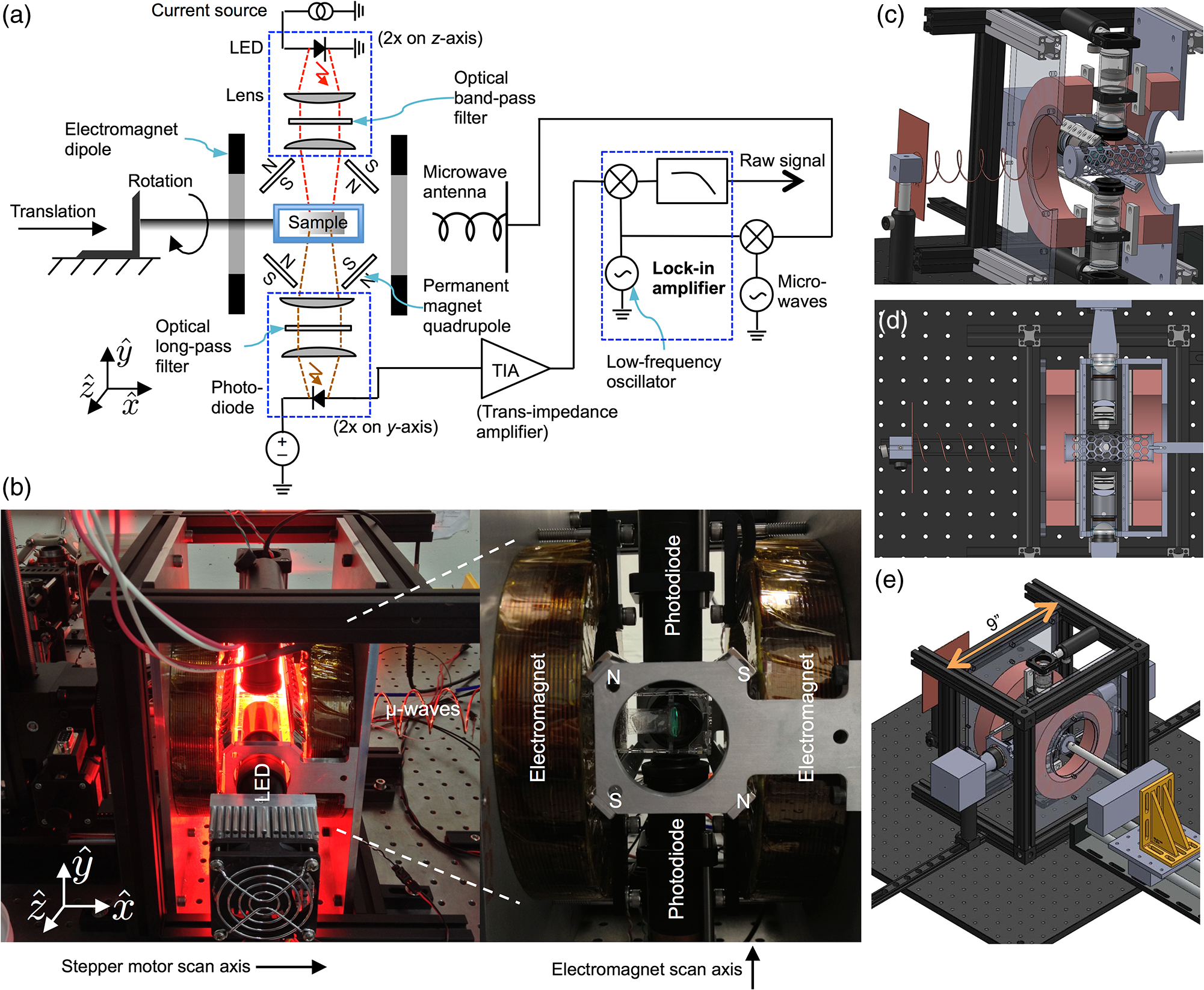

Compared to the first imaging system, there are many improvements in the magnetics. First, the field-free line is generated by four lines of permanent magnets that extend 7 in. along the $\hat{z}$ axis with orientation as shown on the right of Fig. 2(b). This extended the length of the field-free line relative to the first system, in which it was generated by four 1 in. disc magnets in a similar orientation. With a longer field-free line, the PSF of the imaging system is less sensitive to the position of a point of nanodiamonds along the $\hat{z}$ axis. Second, the size of the electromagnets was significantly increased and they were placed further away from the subject than the permanent magnets. By moving the electromagnets further from the subject, the field generated by the electromagnets more closely approximates a dipole (constant) field within the field of view. Although the dipole field points along the axis between the electromagnets (the $\hat{x}$ axis), as one deviates along the $\hat{z}$ axis from $z=0$, the radial component from the electromagnets (i.e., the component of the field projected into the $\hat{y}\hat{z}$ plane) becomes nonzero. As the field-free line is scanned along the $\hat{y}$ axis, this radial component of the dipole field causes the field-free line to decrease in length, or collapse, about the $\hat{x}\hat{y}$ plane. It is important that the field-free line can be scanned across the full field of view without collapsing because the collapse of the field-free line (or equivalently, the radial component of the electromagnet field) degrades the resolution of the PSF near the periphery of the field of view.

To verify that the field-free line could be scanned sufficiently across the field of view without collapsing, we calculated the magnetic field magnitude across the field of view as a function of electromagnet current. The results (at 3 A electromagnet current) are plotted in Fig. 3. In panel (a), we show the magnetic field magnitude every 5 mm along the $\hat{y}$ axis. The 1 G (0.0001 T) field contour is plotted in red and shown to extend across the sample volume. Although the line starts to decrease in length as it is scanned along the $\hat{y}$ axis, it still covers the full field of view of the imaging system. A contour plot of magnetic field magnitude is shown in panel (b), in the $\hat{x}\hat{y}$ plane.

Fig. 3

Field-free line of imaging system shifted along $\hat{y}$-axis with 3 A in electromagnets. (a) Black cylinder is 30 mm in diameter and represents volume over which field-free line must be rastered without decreasing in length. The 1 gauss contour is shown in red. This contour decreases in length at higher electromagnet currents, yet still extends across the 30 mm diameter field of view. (b) Two-dimensional contour plot of field magnitude at $\mathit{z}=0$.

The imaging system’s optical excitation is provided by two light-emitting diodes (LEDs) (Innovations in Optics, 2900A-100-16-F4, peak wavelength 615 to 620 nm), one on either side of the sample and oriented along the $\hat{z}$ axis. Each optical train provides $\sim 2\mathrm{W}$ optical excitation over a $\sim 12\text{-}\mathrm{mm}$ wide by $\sim 25\text{-}\mathrm{mm}$ high area, after collimating, bandpass filtering (Semrock FF01-615/45-25, 615 nm center wavelength with 45 nm bandwidth), and focusing through a series of spherical and cylindrical lenses. The lens tube has a threaded section to adjust the focus of the excitation spot. It was found that the low-frequency ($\sim 400\mathrm{Hz}$) modulation of the microwaves directly caused the LED output to modulate, thus creating a feed-through signal that overwhelmed the detection of the modulated NV fluorescence at the same frequency. Therefore, a resonant circuit, designed to have high impedance at $\sim 400\mathrm{Hz}$ and formed from the parallel combination of two 10-μF film capacitors and a 10-mH inductor, was placed in series with the LED and the power supply to suppress low-frequency modulation of the LED light. Additional suppression of LED modulation was accomplished with 120 μF across the output of the power supply.

Fluorescence was collected on either side of the sample along the $\hat{y}$ axis, collimated and long-pass filtered (Semrock BLP01-664R-25, 664 nm cutoff), and focused onto a photodiode, with adjacent transimpedance amplifier. The photodiode and preamplifier circuits are identical to the ones used in the first imaging system as described in the Supporting Information of Ref. 5. However, due to the use of high-power radiated microwaves in the new system as compared to the local, near-field excitation used in the first system, we placed the photodiode and preamplifier circuits in a shielded enclosure with a copper mesh optical window that prevented direct feed-through of the microwave modulation onto the signal.

The outputs of the transimpedance amplifiers were separately amplified by low-noise voltage preamplifiers (Stanford Research Systems SR560) and digitized at 125 KHz by a data acquisition card (National Instruments PCIe-6321). Microwaves were generated by an analog signal generator (Agilent E8257D) set to 2.872 GHz and $-3\mathrm{dBm}$ output power (the reason for using 2.872 GHz, rather than the zero-field frequency of 2.869 GHz, is explained in Fig. 5). After chopping with a PIN switch (Mini-Circuits ZASWA-2-50DR+) at 406 Hz (the resonance frequency of the tank circuit used to suppress excitation intensity fluctuations), the microwaves were amplified by a high-power amplifier (Mini-Circuits ZHL-16W-43-S+) to provide $\sim 8\mathrm{W}$ of microwave power that was partially directed toward the sample with a helical antenna. A LabVIEW program scanned the field-free line relative to the sample by varying the electromagnet current via an analog output board (National Instruments PCI-6722) connected to the magnet power supplies and by varying the position of the translation stage. The program also synchronously detected the resulting changes in fluorescence with a software-based lock-in detection scheme.

2.3.

Sample Preparation and Imaging

Individual nanodiamond “phantoms,” or test targets for imaging, were prepared starting with $2\times 2\mathrm{mm}$ squares of double-sticky tape. A 5 μl drop of nanodiamond solution containing 5 μg of 100-nm nanodiamond particles, prepared as in Refs. 15 and 19, was placed on each square of double-sticky tape and allowed to dry under a heat lamp. The process was repeated twice for a total of 15 μg of nanodiamond on each square. The squares were arranged into patterns as photographed in Figs. 4(a) and 4(f) and supported by a piece of optical sealing tape held by an acrylic mount.

Fig. 4

Image data from second imaging system. (a), (b), (j), (c), and (k) Photos of phantom, raw image data, surface plot of data, deconvolved image, surface plot of deconvolved image for phantom in (a). (f), (g), (l), (h), and (m) Same, for phantom in (f). (d) Line scans through images in (b) and (c). (i) and (e) PSF and surface plot of PSF.

3.1.

Images

The raw images of the phantoms, shown in Figs. 4(b) and 4(g), are both recorded with $0.25\times 0.25\mathrm{mm}$ pixels and 0.5 s of integration at each pixel. The former is $20\times 30\mathrm{mm}$ and the latter is $30\times 40\mathrm{mm}$. The deconvolved images, in Figs. 4(c) and 4(h), respectively, are obtained from the raw images using DeconvolutionLab²⁰ in ImageJ, by applying 1000 iterations of the Tikhonov–Miller deconvolution algorithm with regularization parameter 0.0001 and with a positivity constraint enforced on the solution. (Tikhonov–Miller deconvolution is essentially a minimum-norm least squares fit to the data; that is, it solves $\underset{\mathbf{x}}{\min }({\Vert A\mathbf{x}\mathrm{\text{–}}\mathbf{b}\Vert }^2+\eta {\Vert \mathbf{x}\Vert }^2)$, where $\mathbf{x}$ represents the deconvolved image, $\mathbf{b}$ represents the measured data, $\eta$ is the regularization parameter, and $A$ is the system matrix that represents the imaging system’s PSF.) Figure 4(d) is a line-scan along the diagonal of both the raw image (b) and the deconvolved image (c) of the first phantom, illustrating the efficacy of the deconvolution. However, note that even without deconvolution, the raw images are accurate visual representations of the phantoms.

The PSF of the second imaging system, as shown in Figs. 4(e) and 4(i), was obtained directly from ODMR data of the NV-nanodiamonds. The permanent magnets were removed from the imaging system to separately measure the influence of magnetic field and position-dependent excitation intensity on the PSF; it was reasonably assumed that these effects independently influenced the PSF. Two squares of nanodiamond-coated double-sticky tape were placed adjacent to each other to make a $2\text{-}\mathrm{mm}\text{wide}(\hat{x}\text{direction})\times 4\text{-}\mathrm{mm}\text{high}(\hat{y}\text{direction})$ test target.

3.2.

Obtaining the PSF

Two types of scans were performed to obtain the PSF. The first, measuring the influence of magnetic field, is illustrated in Fig. 5(a) and consisted of sweeping the magnetic field $B$ from $-200\mathrm{G}$ to 200 G and observing the changes in fluorescence, with microwaves on at 2.872 GHz. Values for $\pm B$ were averaged, and a ninth-order polynomial was fitted to the resultant plot. We assumed that the magnetic field gradient $G$ of the second imaging system was constant (due only to a quadrupole term), so the field magnitude a distance $r$ away from the field-free line was given by $B=Gr$, and the polynomial could be evaluated as a function of $r$ to calculate the dependence of the PSF on the spatially varying magnetic field. The peak modulation of the fluorescence was roughly 0.1% of the background; background sources included NV fluorescence, fluorescence of material within the optical pathway (including the double-sticky tape), and feed-through of out-of-band LED light through the optical interference filters.

Fig. 5

(a) Magnetic field dependence of ODMR at 2.872 GHz (imaging frequency) and 2.869 GHz (zero-field NV spin resonance frequency) creates plots that are equivalent to the PSF in a quadrupolar magnetic field (linear gradient). Note that the shape of the data is almost the same at each frequency, with the exception that the signal at 2.872 GHz is $1.73\times$ the signal at 2.869 GHz, and the bulk of the signal energy is in the central peak at the higher frequency. (The essentially identical data from negative and positive field amplitudes were combined to enhance the SNR.) (b) Measured ODMR data of NVs showing both magnetic field and microwave frequency dependence (measured with original system). Horizontal bars represent cuts through data corresponding to plots in (a), illustrating the higher signal and smaller tails at 2.872 GHz. (c) The simulated ODMR data, which corresponds to the measured data in (b).

To estimate the profile of the LED excitation spot and include it in the PSF, a second scan was performed by translating the test target (in the $\hat{x}$ direction, using the translation stage) across the excitation spot. A sixth-order polynomial was fitted to this ODMR dataset as a function of position of the test target relative to the LED excitation spot. Because the test target had an extent of 2 mm in the scan direction, it was necessary to deconvolve the recorded data with a 2-mm wide “box” (Π-shaped) function to obtain a better estimate of the actual LED profile. Finally, the contributions to the PSF from the spatially varying magnetic field and the spatially varying LED excitation profile were multiplied together, at each point in space, to obtain the PSF.

3.3.

Influence of Microwave Frequency

To illustrate the advantage of imaging at 2.872 GHz instead of at 2.869 GHz (the zero-field NV spin transition frequency used in the first experiments described in Ref. 5), we show a plot of the PSF at both frequencies in Fig. 5(a). At 2.872 GHz, the signal strength is $1.73\times$ higher than at 2.869 GHz, yet the spatial resolution is almost the same (1.2 versus 1.0 mm FWHM). Most notably, at 2.872 GHz, the PSF does not have the broad tails it has at 2.869 GHz. These broad tails concentrate the energy of the PSF at low spatial frequencies, thus reducing the contrast of images acquired at the lower microwave frequency. Thus, imaging at 2.872 GHz better preserves the higher spatial frequencies of the nanodiamond distribution within the subject during the imaging process.

To understand why the broad tails of the PSF are not present at 2.872 GHZ, in Fig. 5(b) we show a plot of the measured ODMR data of the nanodiamonds versus microwave frequency and magnetic field. This plot was obtained using a modified version of the experimental apparatus as described in Ref. 5; essentially, a $2\times 2\mathrm{mm}$ square of double-sticky tape covered with 10 μg of 100 nm nanodiamonds was illuminated with red light at $\sim 620\mathrm{nm}$ and an optical intensity of ${\sim 1\mathrm{W}\mathrm{cm}}^{-2}$. Microwaves were applied via a $\sim 12\mathrm{mm}$ square loop that surrounded the piece of double-sticky tape, and the microwaves were chopped at 379 Hz. The modulation in fluorescence was measured synchronously as a function of microwave frequency (from 2.819 to 2.919 GHz in 1-MHz steps) and magnetic field (from $-40\mathrm{G}$ to 40 G in 1-G increments), with the magnetic field along the $\hat{z}$̂ axis and the microwave field along the $\hat{x}$ axis.

We indicate two cuts through the plot in Fig. 5(b), one at each of the microwave frequencies used to obtain the plots in Fig. 5(a). At zero magnetic field, we see evidence of two spin transitions at slightly different frequencies. These are transitions between the $m_s=0$ and $m_s=\pm 1$ states, where strain within the nanodiamonds has caused the $m_s=\pm 1$ states to split and hybridize as states that transform as $X$ (slightly higher in energy, by convention) and $Y$ (slightly lower in energy). At 2.869 GHz, the microwave frequency is exactly in between the two spin transitions, within the anti-crossing between the two hybridized states, so the observed signal is weaker than at 2.872 GHz, which overlaps more directly with one of the spin transitions. Also, the broad tails of the PSF are lower in amplitude at the higher frequency because the anti-crossing blue-shifts with applied magnetic field; the 2.872 GHz frequency cuts into the anti-crossing, whereas the 2.869 GHz does not (it actually comes out of the anti-crossing at higher magnetic fields, hence generating the broad tails). We can understand the observed plot by calculating the expected ODMR lineshape of the NVs in nanodiamond powder, as we do in the next section, starting from the NV spin Hamiltonian.

3.4.

Model of ODMR Lineshape

Starting from the NV spin Hamiltonian, we calculated the ODMR lineshape that was observed in Fig. 5(b); the calculation results are presented in Fig. 5(c). The NV Hamiltonian, combining zero-field splitting (first two terms) and the Zeeman interaction (final term), is shown in the following equation:

The energy levels and energy eigenstates for a single NV depend on the orientation of the NV axis with respect to the applied magnetic field. However, the ODMR lineshape includes contributions from an ensemble of NVs randomly distributed in solid angle and with randomly distributed strain $E$. For a given member of the ensemble, we obtain three states (with three corresponding energy levels) when solving the Hamiltonian. Call them $|0\rangle$, $|1\rangle$, and $|2\rangle$, with $|0\rangle$ consisting primarily of the $m_s=0$ state and $|1\rangle$ and $|2\rangle$ consisting of superpositions of the $m_s=\pm 1$ states. Label their eigenenergies as $E_0$, $E_1$, and $E_2$, respectively, so the two spin transitions occur at the following microwave frequencies: ${\omega }_1=(E_1-E_0)/\hslash$ and ${\omega }_2=(E_2-E_0)/\hslash$. The Rabi frequency for each transition is

We calculate the lineshape for one of the transitions according to the Bloch equations for a two-level system:²¹

We use $f[h_1(\omega ),h_2(\omega )]=\max [h_1(\omega ),h_2(\omega )]$, a “winner-takes-all” paradigm for selecting which transition out of the two is favored at a given frequency, justified by the fact that we are well into saturation ($4{\mathrm{\Omega }}^2{T}_1{T}_2\gg 1$) and both transitions share the lower $m_s=0$ level. Finally, the ensemble lineshape is calculated by averaging over the strain distribution $p_E(E)$ (modeled as a Gaussian with mean ${\mu }_E$ and variance ${\sigma }_E$) and over the Euler angles:

To create the plot in Fig. 5(c), we use the parameters summarized in Table 1, which have been varied by hand to produce the best qualitative fit to measured data. A quantitative optimization of the parameters was not done, but could potentially be adapted to this framework (see, for example, the Supporting Information in Ref. 22).

Table 1

Parameters used to estimate the NV ODMR powder lineshape depicted in Fig. 5(c).

3.5.

Imaging System Sensitivity

The sensitivity of the current imaging system, calculated from the measured SNR of a known quantity of nanodiamonds and scaled to an SNR of unity, is ${1.6\mathrm{mM}\mathrm{mm}}^3{\mathrm{Hz}}^{-1/2}$. That is, the system can detect a 1.6 mM concentration of carbon atoms filling a millimeter cube volume in 1 Hz of measurement bandwidth. Note that in a biological context, some nanodiamond material may be present in nontargeted regions of the subject, due to the inability to generate perfect contrast biologically. Therefore, the signal of interest is actually the difference in signal intensity between the targeted and nontargeted regions, and the sensitivity will be reduced by the corresponding contrast ratio. For example, a factor of 5 difference in the nanodiamond concentration between targeted and nontargeted regions yields a sensitivity of 80% of the original sensitivity. In addition, the sensitivity decreases with depth into the subject at a rate approximately three times faster than the effective optical attenuation, as described in detail in Ref. 5.

The main noise source is shot noise from the unmodulated fluorescence background, although the calculated sensitivity is $\sim 4\mathrm{dB}$ above the expected shot noise from the background. In addition to noise caused by electrical pick-up, excess noise may be due to sample vibration at the measurement frequency. The sample was supported at the end of a long cantilever to provide travel room for the translation stage. This turned out to amplify vibrations at the measurement frequency, which modulated the DC background and appeared as a stochastic feed-through component (additive noise) on top of the signal.

The first prototype imaging system had a sensitivity and resolution of ${2.2\mathrm{mM}\mathrm{mm}}^3{\mathrm{Hz}}^{-1/2}$ of carbon atoms and $\sim 800\text{micron}$ FWHM, respectively, as calculated in Ref. 5; the sensitivity of the current system improved on the previous system’s sensitivity by $\sim 3\mathrm{dB}$. Numerous sensitivity enhancements that add up to a $\mathrm{29,000,000}\times$ improvement in sensitivity have been explored in the Supporting Information of Ref. 5, with the primary enhancement arising from an increased NV concentration within the nanodiamonds.

While the current system has a spatial resolution of 1.2 mm, the resolution was measured differently than in the first system. In this paper, we quote for the resolution the FWHM of the PSF; the spatial resolution of the system described in our previous paper, with a similar magnetic gradient, was quoted as the FWHM of the PSF’s central peak only. Resolution scales as the inverse of the gradient of the magnetic field magnitude and can be improved by increasing the magnetic gradient. [Scaling the magnetic field by an amount $\alpha$ is equivalent to horizontal scaling of the PSF in Fig. 1(e) by an amount $1/\alpha$].